RHiOTS in practice: the most accurate forecaster is not the most robust

Introduction

A team building a hierarchical forecast usually settles two choices with one benchmark table: which base forecaster to fit, and which reconciliation method to use so its levels add up. Bottom-Up simply sums each aggregate from its own children's forecasts. MinT (minimum trace) [2] instead re-weights every level's forecast using the covariance of past errors, chosen to minimize the combined error across the hierarchy.

Most such tables come from one clean dataset, scored once. They tell a reader which setup won on that dataset, not whether the win would survive a worse one.

We built a framework for that second question at KDD '24, called RHiOTS [1]. It perturbs a real dataset at increasing intensities and re-scores every method on each distorted copy, turning a single number into a curve. Here we apply it to four base forecasters, AutoETS, NBEATS, PatchTST and HINT, on the Australian tourism hierarchy [2], a dataset we have used before on this blog.

The setup that wins on clean data is not the one that holds up. NBEATS, paired with its own best reconciler, gives the most accurate reconciled result in the whole comparison, and also the least robust one. It degrades roughly four times faster under noisy training data than AutoETS's own pick, which starts out less accurate, and falls behind that pick partway through the noise levels we tested.

A team that benchmarked all four on clean data would pick NBEATS, the setup whose accuracy degrades fastest once its training data gets noisier.

We build up to that comparison with AutoETS alone. On clean data, MinT beats Bottom-Up, as our earlier article on this same dataset measured directly. Under noise, that margin shrinks by as much as four fifths at the national total, though MinT never loses its lead.

As always, the code is available on our GitHub.

RHiOTS: stress-testing instead of one-shot benchmarking

RHiOTS perturbs a real, published dataset instead of collecting a new one. Four transformations, jitter, scaling, magnitude warping and time warping, are applied to the bottom-level series at increasing intensity, and every parent series is recomputed by summing its children, so the hierarchy stays coherent by construction.

Forecasting methods are re-scored on each distorted copy, which turns one static benchmark table into a curve: how accuracy, or a reconciliation method's advantage, changes as the data drifts from the one dataset it was tuned on.

This article uses jitter, additive noise on each bottom series, as a stand-in for the most common way real data disappoints a validated model. Next quarter's numbers carry more measurement noise, or more volatile demand, than the historical window a method was chosen on. Take a single region's monthly tourism series. Jitter adds an independent random amount to every month, sized to that region's own historical volatility, and the region's state and country totals move with it, recomputed by simple addition. Applying it at increasing intensity is the whole experiment: fit the same models, reconcile the same way, and watch what happens to the comparison a clean-data table already settled.

Applying RHiOTS: does the clean-data winner survive noisy training data?

Dataset and protocol

We reuse the Australian tourism hierarchy from our reconciliation article: 304 monthly region-by-purpose series (76 regions, 4 travel purposes), aggregating through region, zone and state to a national total. It is 415 series in all, January 1998 to December 2016, from Tourism Research Australia's National Visitor Survey [2]. Forecasts use statsforecast's AutoETS (automated exponential smoothing), reconciled with hierarchicalforecast [3]'s Bottom-Up and MinT (shrinkage) methods, over the same four rolling-origin folds as our reconciliation article.

We jitter only the training history, at RHiOTS's own six intensities and ten random draws per intensity, using the shipped jitter code ported into our own pipeline. The forecast is then scored against the untouched, clean test truth, with the accuracy metric's own scale fixed to the original, unperturbed history throughout. That design answers the practitioner's actual question: my history is noisier than I assumed, does the reconciliation choice still make sense? It also does so without letting the comparison mark its own homework. The evaluation target never sees the injected noise, and the yardstick used to score it never moves either.

Where reconciliation helps in the first place

Before adding any noise, we reproduce our earlier article's own numbers exactly, since this experiment reuses the same dataset, folds and reconciliation code. MinT's accuracy advantage over Bottom-Up on clean data is not spread evenly across the hierarchy. It is largest at the national total, smaller at each level down, and close to zero at the bottom series, where Bottom-Up has nothing left to reconcile away.

A reconciliation method that only helps where there is something to reconcile is exactly what the mechanism predicts. It is worth knowing before the next result, because it is precisely the levels where MinT helps most that turn out to be the least stable.

What happens under noisy training data

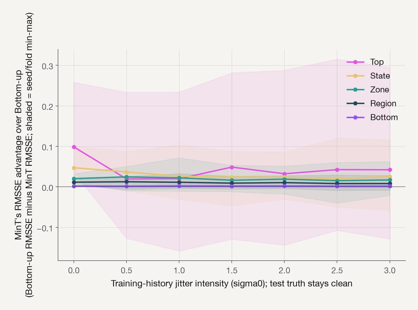
Figure 1 shows the same clean-data gap at zero intensity, then what RHiOTS's stress test does to it. At the national total, even the mildest intensity we tested cuts MinT's edge by roughly four fifths, and the margin never fully recovers, settling into a smaller, noisier band rather than disappearing outright.

The state level's advantage roughly halves over the same range. The bottom level, where the advantage was never large, stays close to flat throughout.

That advantage is specifically over Bottom-Up: the earlier article also found MinT trailing the unreconciled base itself by a wide margin at the national total, so "MinT wins" is about which reconciliation to pick, not that reconciling always beats not reconciling.

A team that picked MinT because it won on a clean validation set would still be right to prefer it here. But the margin it was chosen for is not the margin it should expect once the training data looks less tidy than the set it was tuned on. At the level where MinT's advantage was largest, that margin is also the least dependable one.

Results and discussion

Figure 1 shows MinT's advantage as a single number: the gap between the two methods. A shrinking gap does not say which method is actually robust. It could mean Bottom-Up is getting more accurate, or it could mean MinT is getting less accurate.

We score every forecast with RMSSE, which scales each series' error by its own in-sample seasonal naive error. To tell the two apart, we looked at each method's own score at the national total.

We also added two more hierarchicalforecast reconcilers. WLS (variance) reconciles using only each series' own error variance. Top-down (proportions) has nothing above the national total to disaggregate from, so its curve there sits exactly on Base's, and we leave it out of Figure 2.

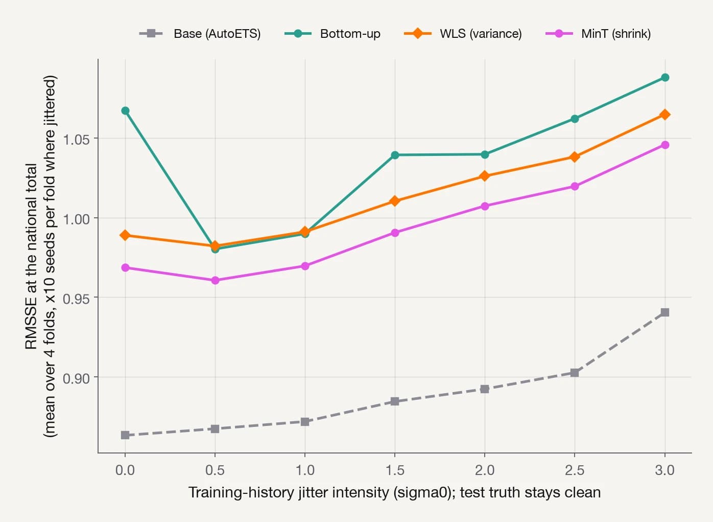
Most of Figure 1's narrowing comes from Bottom-Up getting better at the mildest intensity, not from MinT getting worse. Bottom-Up's own score drops sharply the moment any jitter at all is added, by 6 to 12 percent depending on the fold, then climbs back to land close to where it started. MinT barely moves at that same first step.

This holds in every one of the four folds, so it is not noise, but we cannot yet attribute it to a specific mechanism.

Over the full range, MinT's own RMSSE rises by about 8 percent, almost as much as the unreconciled base forecast, against only 2 percent for Bottom-Up. WLS moves almost exactly like MinT. Even so, MinT's RMSSE stays below Bottom-Up's at every intensity we tried.

The margin held throughout our test, but a one-shot benchmark could not have told you that in advance, or how much it would move.

Does this hold with other base forecasters?

We repeated the sweep with three more base forecasters: NBEATS [4], PatchTST [5] and HINT [6]. Wherever the model allowed it, we matched the AutoETS arm's rigor: the same six-point jitter grid, the same ten seeds per intensity, the same four folds, even the same noise draws. Only the base forecaster differs between runs.

HINT reconciles differently from the other three. NHITS, its base model, trains on all 415 series with a probabilistic loss, and coherence is imposed only at prediction time. It also supports only two of our three reconcilers: Bottom-up, and a variance-weighted method (MinTraceWLS) built on the same idea as WLS (variance).

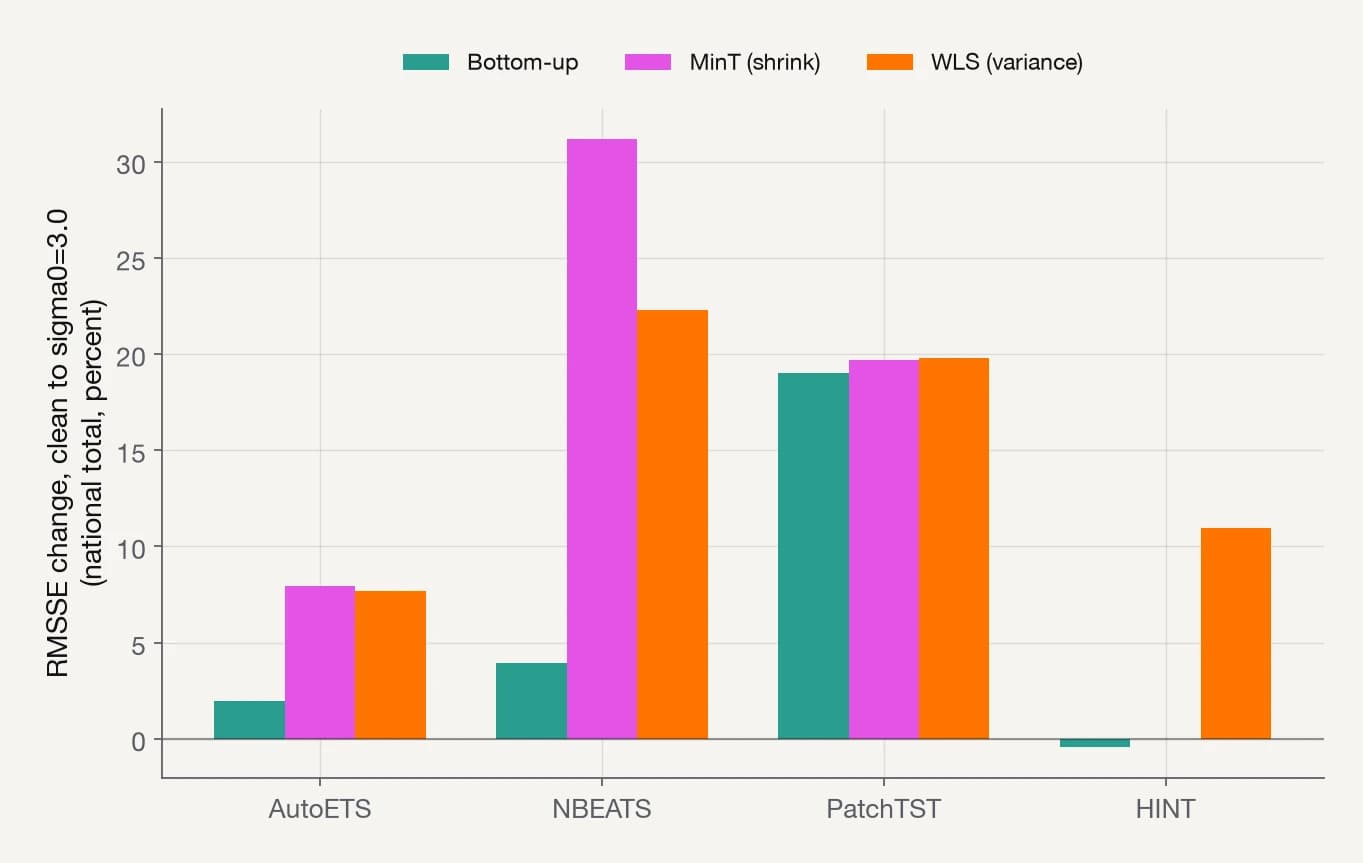
Figure 3 shows that the AutoETS result only partly generalizes. Bottom-Up's own resilience is real for three of our four base forecasters and gone with PatchTST. What does not generalize is the size of the resilience gap.

NBEATS agrees with AutoETS, more sharply. Its MinT score rises 31 percent from clean to the noisiest run we tested, against 4 percent for Bottom-Up. HINT follows the same pattern, its Bottom-Up score barely moving while its MinTraceWLS score rises 11 percent.

PatchTST erases the gap instead of reversing it. Its own RMSSE, Bottom-Up's, MinT's and WLS's all rise by about 19 to 21 percent, so whichever reconciler you pick costs you almost the same under noise.

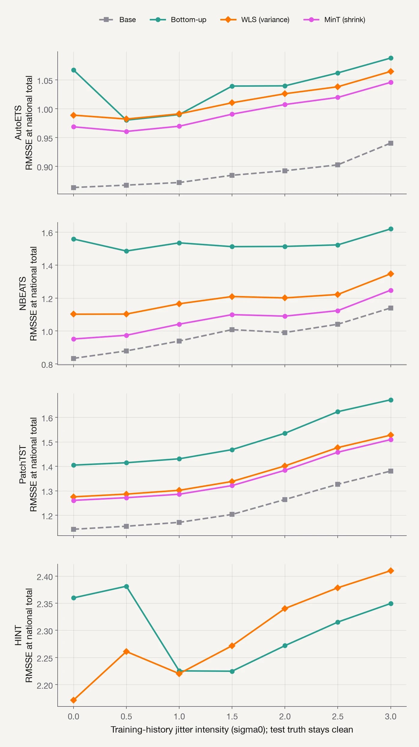
Figure 4 shows where those scores sit. A WLS-family reconciler is more accurate than Bottom-Up at every intensity we tested for AutoETS, NBEATS and PatchTST. HINT is the exception. Its MinTraceWLS wins only at the two mildest intensities, then Bottom-Up takes over for the rest of the range.

HINT also starts from a different place. Its best run, at 2.17, is worse than NBEATS's worst, at 1.62.

Both the reconciler and the noise level change the answer, and neither a clean-data benchmark nor a stress test run against one base forecaster tells you by how much.

Lining up each model's own best pick makes the trade-off visible on one chart. Figure 5 tracks each forecaster's clean-data winner, MinT (shrink) for AutoETS, NBEATS and PatchTST, MinTraceWLS for HINT, across the full jitter range.

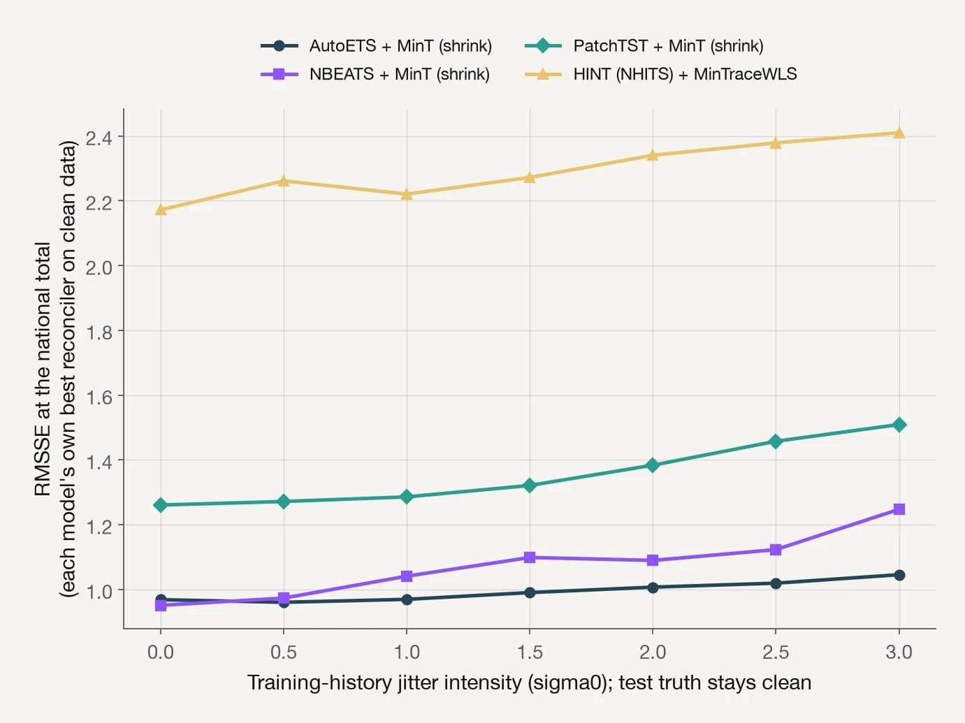
AutoETS's line is the flattest of the four. NBEATS's starts lowest of all, its clean-data RMSSE of 0.95 is the lowest starting point of the four, but its line is also the steepest: it crosses above AutoETS's at the very first jittered point, sigma0=0.5, and keeps climbing. PatchTST's line sits above both, rising almost as fast as NBEATS's. HINT's sits apart from the other three, more than a full point of RMSSE higher throughout.

NBEATS wins on clean data. AutoETS wins on resilience, degrading roughly four times more slowly under jitter despite starting from a worse number, the gap the introduction pointed to.

Conclusion

RHiOTS turns "which setup wins" from a one-shot answer into a question with a condition attached. On the Australian tourism hierarchy, NBEATS's best pick is the most accurate reconciled setup in this comparison, and also the least robust. It degrades roughly four times faster under jitter than AutoETS's own pick, which started out worse.

A clean-data benchmark cannot tell those two apart. The team that skips the stress test picks NBEATS, trusting a lead the data cannot actually promise.

Our single-model worked example points the same way. With AutoETS, MinT's advantage over Bottom-Up is real and concentrated at the aggregate levels. It shrinks by as much as four fifths at the national total, and roughly half at the state level, once the training data is noisier than the data it was tuned on, though MinT never loses it. Most of that narrowing happens at the mildest jitter we tested, and traces to Bottom-Up's own accuracy improving there, in every fold, not to MinT getting worse.

That result generalizes less cleanly. Swapping AutoETS for NBEATS confirms the resilience gap, more sharply, while PatchTST erases it. HINT is far behind the other three on raw accuracy throughout, and even which reconciler wins on accuracy flips partway through the jitter range. Nothing about which reconciler wins held across all four base forecasters we tried.

We recommend stress-testing the whole setup, base forecaster included, rather than the reconciler alone. That is the confidence a stress test buys a practitioner: not just which method wins today, but which one keeps winning once the data stops cooperating.

References

[1] Roque, L., Soares, C., & Torgo, L. (2024). RHiOTS: A Framework for Evaluating Hierarchical Time Series Forecasting Algorithms. Proceedings of the 30th ACM SIGKDD Conference on Knowledge Discovery and Data Mining (KDD '24). https://doi.org/10.1145/3637528.3672062

[2] Wickramasuriya, S. L., Athanasopoulos, G., & Hyndman, R. J. (2019). Optimal forecast reconciliation for hierarchical and grouped time series through trace minimization. Journal of the American Statistical Association, 114(526), 804-819. https://doi.org/10.1080/01621459.2018.1448825

[3] Olivares, K. G., Garza, A., Luo, D., Challú, C., Mergenthaler, M., Ben Taieb, S., Wickramasuriya, S. L., & Dubrawski, A. (2022). HierarchicalForecast: A reference framework for hierarchical forecasting in Python. arXiv:2207.03517

[4] Oreshkin, B. N., Carpov, D., Chapados, N., & Bengio, Y. (2020). N-BEATS: Neural basis expansion analysis for interpretable time series forecasting. International Conference on Learning Representations (ICLR 2020). arXiv:1905.10437

[5] Nie, Y., Nguyen, N. H., Sinthong, P., & Kalagnanam, J. (2023). A Time Series is Worth 64 Words: Long-term Forecasting with Transformers. International Conference on Learning Representations (ICLR 2023). arXiv:2211.14730

[6] Olivares, K. G., Luo, D., Challu, C., La Vattiata, S., Mergenthaler, M., & Dubrawski, A. (2023). Hierarchically Coherent Multivariate Mixture Networks. arXiv:2305.07089

All images are by the authors unless noted otherwise.