Forecast Reconciliation on the Australian Tourism Hierarchy: MinT, Bias and Chronos-Bolt

Introduction

A demand plan is read at several levels at once. Finance budgets the national total and operations staffs each state or each warehouse. The people closest to the customer work with the smallest series: one product in one store, or, in the tourism data we use here, the visitor nights in one region for one purpose of travel.

When each level is forecast on its own, the numbers do not add up. The small forecasts sum to one figure, the forecast of the total says another, and the planning meeting opens with an argument about which one to believe.

Forecast reconciliation ends the argument. It adjusts the forecasts so that they add up, the way the actuals do. The methods that do this well promise something more: a set of forecasts that is more accurate than the ones you started with, because each level's forecast holds information the others lack. Hyndman et al. [1] showed the gain on Australian tourism data, Wickramasuriya et al. [2] sharpened it into a method called MinT, and both results are now repeated in every tutorial on the subject.

In the planning stacks we work on, the promise is read as a guarantee, and it does not survive contact with the numbers. The textbook example by Hyndman and Athanasopoulos [3], on the quarterly version of the same tourism survey, prints a table in which the national total's RMSE gets 25% worse after MinT. Its text adds only that reconciliation "usually improves" the forecasts "for almost all levels". A planner who watches the total get worse stops trusting the reconciled plan, and the whole exercise is undone in a spreadsheet.

In our view, the promise and the table are both right, because the guarantee behind reconciliation is narrower than its usual reading. Panagiotelis et al. [4] proved that the projection behind the optimal family cannot increase the forecast error summed over every series, in the method's own measure of distance. The theorem says nothing about a single level, a single series, a forecast that came from outside the model, or a biased forecast, which are the four cases a planner deals with every week.

In this article, we build the concepts up from a retailer with two stores, so that the reader sees what each method does to the numbers before any notation arrives. After that, we run every method on the monthly tourism hierarchy, the same 304 bottom series we used in our Chronos and FORGE posts, and measure each of the four cases.

We find that MinT is the most accurate method on average and that it makes the national total 12% worse on average, and worse in every fold, because it inherits the bias of the small series. Correcting that bias first turns the loss into a gain when every series is corrected, at a cost to the small series, and recovers most of the loss when only the aggregates are. Finally, we reconcile zero-shot forecasts from Chronos-Bolt, where the first surprise is that the point forecast is a median.

As always, the code is available on our GitHub.

A hierarchy, and forecasts that add up

Imagine a retailer with two stores in Portugal, one in Lisbon and one in Porto. The stores are the children in the hierarchy and Portugal is the parent, and the actuals always add up: if Lisbon sold 60 units and Porto sold 30, Portugal sold 90. Forecasts made one series at a time are under no such obligation.

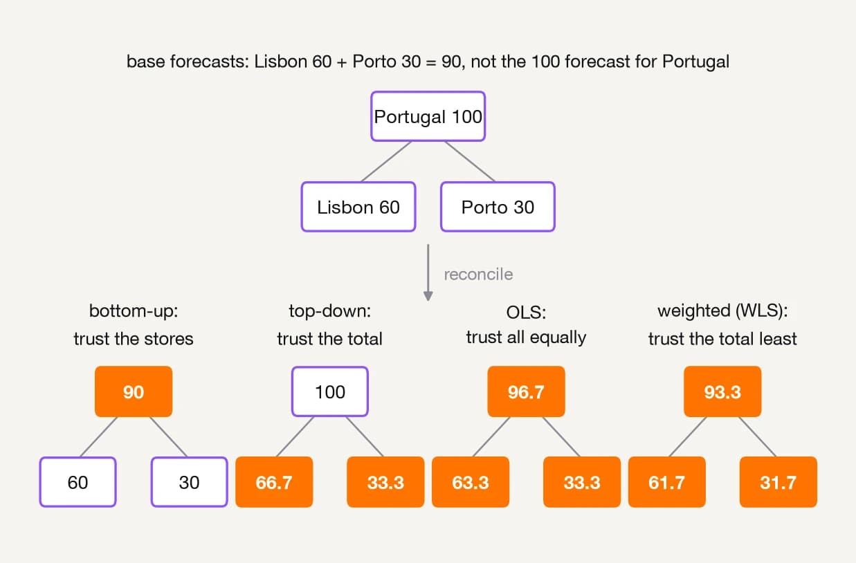
Suppose the Lisbon store forecasts sales of 60 and the Porto store 30, while the retailer has independently forecast Portugal at 100. Each number may be reasonable on its own, and together they do not agree: the two stores add up to 90, not 100.

We call forecasts that add up coherent, and the retailer's three forecasts are incoherent. A planner who meets the disagreement has a choice to make: which of the three numbers to move, and by how much.

Every reconciliation method is one answer to that question, and the rest of the article is about which answers are good ones.

The bookkeeping of "adds up" is a matrix. A summing matrix S has one row per series and records which children each series adds up, so multiplying it by the vector of children returns every series at once. Equation 1 shows it for the retailer: multiply the two store forecasts by S and the three coherent numbers come out, Portugal included.

In general, with b the vector of bottom series and y the vector of all series, y = S b. Forecasts are coherent when they satisfy Equation 1. Base forecasts, produced one series at a time, we write ŷ.

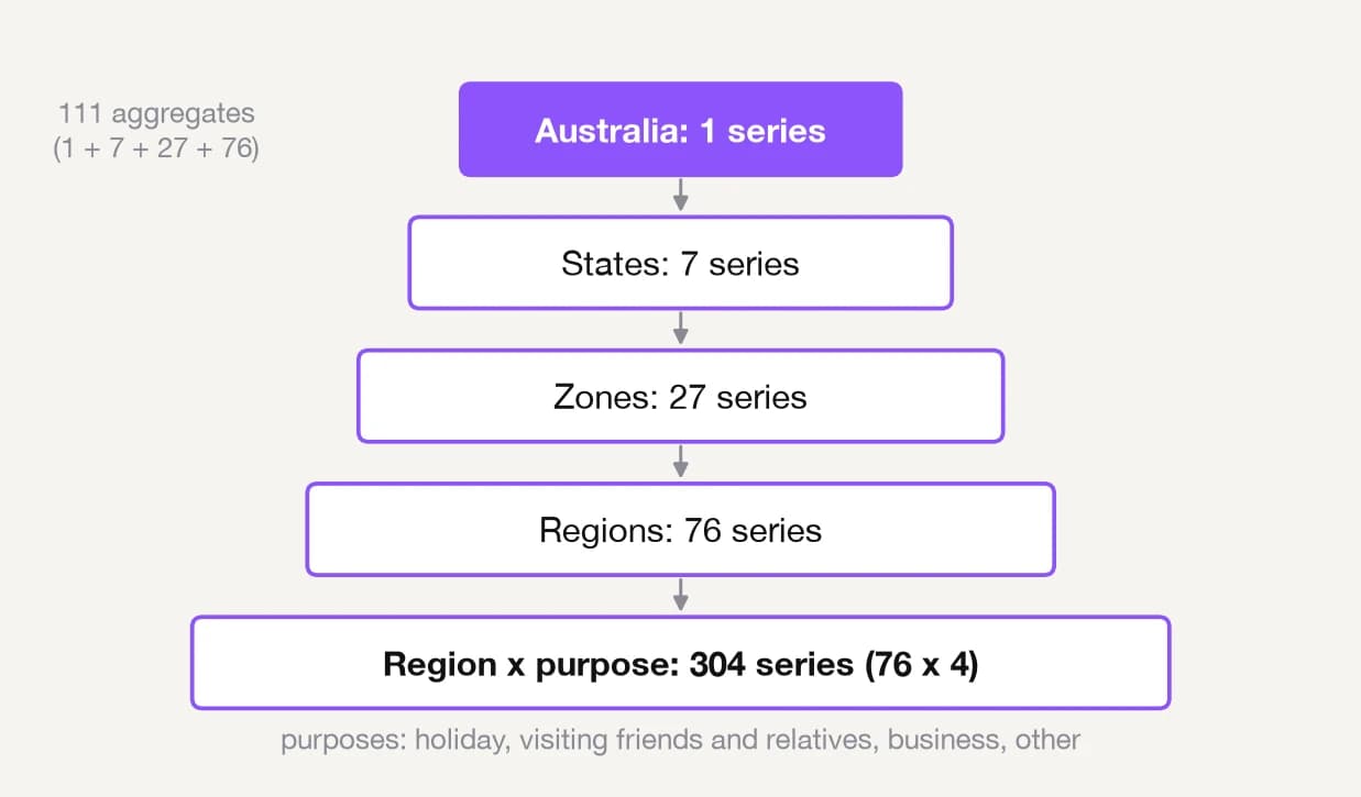
The real hierarchy we forecast later is the Australian tourism survey, shown in Figure 1. It divides the country into seven states and territories, 27 zones and 76 regions, and every trip has one of four purposes: holiday, visiting friends and relatives, business, or other.

That gives 304 bottom series (regions times purposes) and 111 aggregates, 415 series in total, and an S with one row for each of them that plays the same role as the three-row one above.

In our data, the sum of the 304 bottom forecasts differs from the forecast of the total by 1.6% to 4.8%, depending on the year, in the measure we reuse for Chronos-Bolt below.

Note that the full dataset also aggregates by purpose, which turns the tree into a grouped structure of 555 series in which every bottom series belongs to two hierarchies, one geographic and one by purpose. A retailer's store by product is a grouped structure too, and we return to it in the experiments.

Bottom-up, top-down and middle-out

The simplest answers to the planner's question keep one level of the hierarchy and derive the others from it.

Bottom-up trusts the stores. It keeps Lisbon at 60 and Porto at 30, then calculates the Portugal total from those forecasts:

Portugal = Lisbon + Porto = 60 + 30 = 90

The original Portugal forecast of 100 is discarded and replaced with 90. It is how a company budget is built from team submissions: each team provides its own number and head office adds them up. The idea is to trust the most granular forecasts and aggregate upward.

Top-down trusts the total. It keeps Portugal at 100 and splits it between the stores in proportion to their own forecasts:

Lisbon = 100 × 60/90 = 66.7

Porto = 100 × 30/90 = 33.3

The shares can be historical or, as in Athanasopoulos et al. [5] and in our runs, the shares implied by the base forecasts in each month (forecast proportions). Its idea is the reverse of bottom-up: trust the aggregate and hand it down by shares. Middle-out keeps one level in the middle, in our case the states of the tourism hierarchy, sums upward and splits downward.

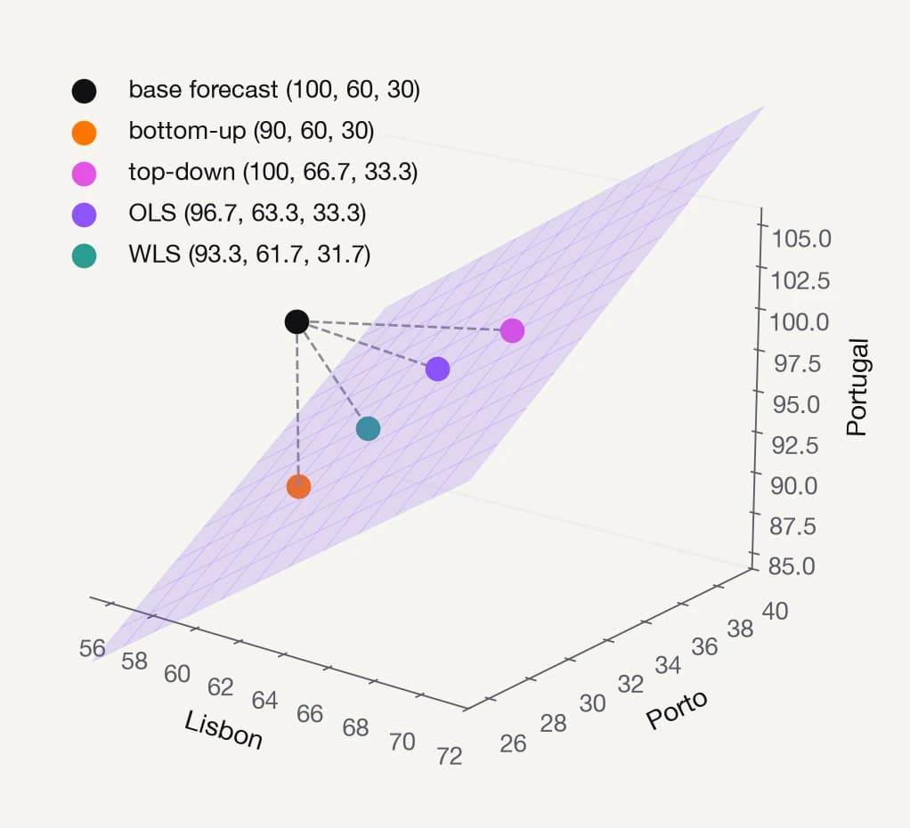
Bottom-up and top-down with fixed proportions can be written as ỹ = S P ŷ (Equation 2), where P is a matrix that produces bottom-level values from ŷ. For the retailer, bottom-up's P has two rows, (0 1 0) and (0 0 1): it reads the two store forecasts and ignores Portugal's. In general it is a zero block next to an identity, and S P is a projection onto the coherent set, which Figure 3 pictures.

Top-down's P has rank one, since every bottom value is a share of one number, and Hyndman et al. [1] showed that it is biased at every disaggregated level even when the base forecasts are unbiased. With forecast proportions it is not even linear in ŷ.

Note that top-down and middle-out also need a tree. In a grouped structure there is no single level to split from, so the hierarchicalforecast library [6] refuses to run them on our 555-series data. Bottom-up works everywhere, which is why it remains the default in most planning systems, and the experiments show what that default costs.

Optimal reconciliation: OLS, WLS and MinT

The optimal family refuses to throw any forecast away. Think of the three forecasts as three noisy readings of the same two underlying numbers, the stores' sales, taken with instruments of different precision, since Portugal's forecast is a reading of their sum. The right combination uses all three readings and leans on the precise ones.

If we trust the three readings equally, the fair move is to spread the discrepancy of 10 evenly, a third each:

Portugal = 100 − 3.33 = 96.67

Lisbon = 60 + 3.33 = 63.33

Porto = 30 + 3.33 = 33.33

The three numbers add up again, and every forecast moved by the same amount.

Knowing that Portugal's forecast errors are four times as variable as a store's changes the answer. Portugal should absorb most of the adjustment, two thirds of it, and each store a sixth:

Portugal = 100 − 6.67 = 93.33

Lisbon = 60 + 1.67 = 61.67

Porto = 30 + 1.67 = 31.67

The idea is to trust every forecast in proportion to its precision and move the least trusted ones most. Figure 2 shows the retailer on the tree, before and after each method, and the pattern to notice is that every method moves a different number.

Hyndman et al. [1] arrived at the equal-trust answer by treating Equation 1 as a regression, with ŷ as noisy observations of S b, and solving it by ordinary least squares (OLS), which gives P = (SᵀS)⁻¹Sᵀ.

Wickramasuriya et al. [2] asked instead for the P that minimises the trace of the covariance of the reconciled errors, which is the sum of every series' error variance after reconciliation, among all unbiased linear reconciliations, hence Minimum Trace (MinT). The answer is Equation 3, where W is the covariance of the base forecast errors.

Equation 3 is the weighted version of the retailer's example. It projects ŷ onto the coherent set, orthogonally in the geometry defined by W⁻¹. Series with a large error variance are cheap to move and series with a small one are expensive, so the incoherence is absorbed where the forecasts are least trusted.

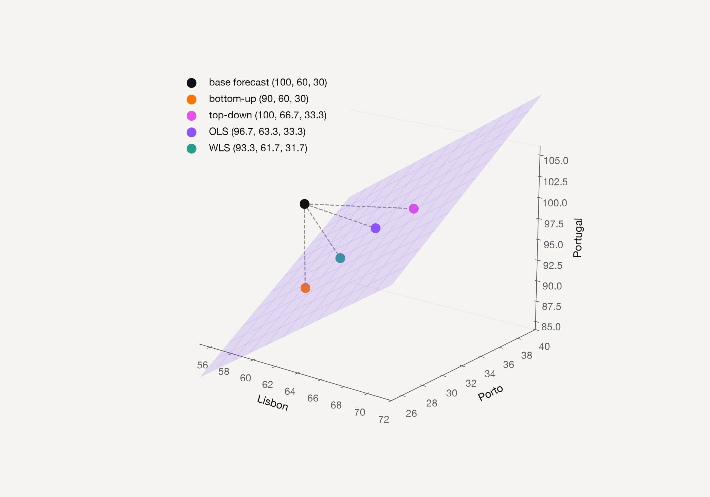
Figure 3 shows the same example geometrically. With Portugal and its two stores, the coherent forecasts form a plane, the base forecast sits off it, and each method lands on a different point of the plane.

In our experiments, the members of the family differ only in W. OLS uses the identity. Variance-scaled WLS [7] uses the diagonal of the in-sample residual variances. Structural WLS [8] uses the number of bottom series under each node and needs no residuals, which is why Wickramasuriya et al. [2] suggest it for judgmental forecasts.

MinT uses the full covariance, shrunk toward its diagonal with the Schäfer and Strimmer estimator [9], because a sample covariance of 415 series estimated from about 200 residuals is singular, and shrinking it toward the diagonal makes it invertible.

Panagiotelis et al. [4] proved what this construction guarantees. The truth y is coherent and ỹ is the projection of ŷ onto the coherent set, so ỹ is never further from y than ŷ is, in the W⁻¹ geometry. For OLS that distance is the plain sum of squared errors over all 415 series.

The guarantee is about the sum, and a sum can fall while some of its terms rise, in the way that a class average can go up while several students' marks go down. Three predictions follow about what the guarantee leaves out, and we test them in this order:

1. Series that were already forecast well relative to their neighbours should lose, because the projection moves them toward worse information.
2. A foreign forecast at one level should pull every other level in its direction, and the weights can limit the damage only if the residuals reveal the change.
3. A bias in the base forecasts should be redistributed but never removed, because W describes variances and not means.

Reconciliation on the Australian tourism hierarchy

In this section, we reconcile AutoETS forecasts of the tourism hierarchy with all seven methods and read the results by level, by series, and under a foreign forecast at one level.

Data and protocol

The data are monthly visitor nights, the nights Australians spend away from home, in thousands, from January 1998 to December 2016. They were assembled by Wickramasuriya et al. [2] from Tourism Research Australia's National Visitor Survey and are distributed with the datasetsforecast package.

The evaluation is a rolling origin with four folds: each fold trains on every month before its cutoff (January 2013, 2014, 2015 or 2016) and tests on the 12 months that follow. Our base model is AutoETS, the automatic exponential smoothing (ETS) model selection in statsforecast, one model per series, with the in-sample fitted values kept for W.

We measure accuracy with the root mean squared scaled error (RMSSE): the RMSE of each series over the 12-month test window, divided by the in-sample RMSE of the seasonal naive forecast.

The scaling makes a national total in the tens of millions of nights comparable with a region-by-purpose series in the thousands. Finally, we report level means of the per-series RMSSE and their change relative to the base forecasts, averaged over folds.

We start by loading the data and restricting it to the geographic tree:

import numpy as np
import pandas as pd
from datasetsforecast.hierarchical import HierarchicalData
from hierarchicalforecast.core import HierarchicalReconciliation
from hierarchicalforecast.methods import BottomUp, MiddleOut, MinTrace, TopDown
from statsforecast import StatsForecast
from statsforecast.models import AutoETS, SeasonalNaive

import utils

HORIZON = 12
CUTOFFS = ["2013-01-01", "2014-01-01", "2015-01-01", "2016-01-01"]
TREE_LEVELS = ["Country", "Country/State", "Country/State/Zone",
               "Country/State/Zone/Region",
               "Country/State/Zone/Region/Purpose"]

Y_df, S_df, tags = HierarchicalData.load("./data", "TourismLarge")
Y_df["ds"] = pd.to_datetime(Y_df["ds"])
tags = {level: tags[level] for level in TREE_LEVELS}
keep = np.concatenate(list(tags.values()))
Y_df = Y_df[Y_df["unique_id"].isin(keep)]
S_df = S_df.loc[S_df.index.isin(keep)].reset_index(names="unique_id")

print(f"{Y_df['unique_id'].nunique()} series, {Y_df['ds'].nunique()} months, "
      f"S is {S_df.shape[0]} x {S_df.shape[1] - 1}")

415 series, 228 months, S is 415 x 304

We define the seven methods in one list, with the states as the middle level and the default shrinkage for MinTrace:

reconcilers = [
    BottomUp(),
    TopDown(method="forecast_proportions"),
    MiddleOut(middle_level="Country/State",
              top_down_method="forecast_proportions"),
    MinTrace(method="ols"),
    MinTrace(method="wls_struct"),
    MinTrace(method="wls_var"),
    MinTrace(method="mint_shrink"),
]

For each fold, we fit the base models, keep their fitted values (the residuals from which W is estimated in MinTrace) and reconcile every method at once:

results = []
for cutoff in CUTOFFS:
    cutoff = pd.Timestamp(cutoff)
    end = cutoff + pd.DateOffset(months=HORIZON)
    train = Y_df[Y_df["ds"] < cutoff]
    test = Y_df[(Y_df["ds"] >= cutoff) & (Y_df["ds"] < end)]

    sf = StatsForecast(models=[AutoETS(season_length=12)], freq="MS",
                       n_jobs=-1, fallback_model=SeasonalNaive(season_length=12))
    Y_hat = sf.forecast(h=HORIZON, df=train, fitted=True)
    Y_fitted = sf.forecast_fitted_values()

    hrec = HierarchicalReconciliation(reconcilers=reconcilers)
    Y_rec = hrec.reconcile(Y_hat_df=Y_hat, Y_df=Y_fitted, S_df=S_df, tags=tags)

    scale = utils.seasonal_naive_scale(train)
    methods = [c for c in Y_rec.columns if c not in ("unique_id", "ds", "y")]
    table = utils.rmsse_table(Y_rec, test, scale, methods)
    table["cutoff"] = cutoff
    results.append(table)

The helpers in utils compute the seasonal naive scale and the per-series RMSSE. After that, we average the per-series RMSSE by level, method and fold:

results = pd.concat(results)
results["level"] = results["unique_id"].map(utils.level_map(tags))
by_level = (results.groupby(["level", "method", "cutoff"])["rmsse"].mean()
                   .groupby(["level", "method"]).mean().unstack())
change = by_level.sub(by_level["AutoETS"], axis=0)
change = 100 * change.div(by_level["AutoETS"], axis=0)

Accuracy by level

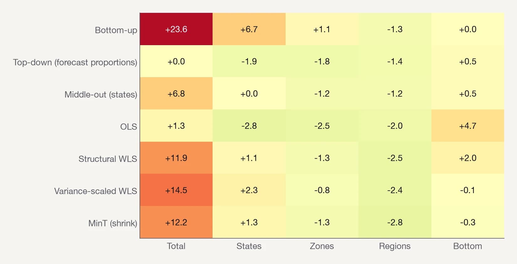
Figure 4 shows the change in RMSSE relative to the base forecasts for every method and level, and its pattern is the article in one picture. The regions improve under every method, by one to three percent, and every method except top-down makes the national total worse.

Averaged over every series, not over the five level means in the figure, we find that MinT is the most accurate method, 0.8% better than the base forecasts and better in every fold. Its total is 12% worse on average and worse in every fold, by 3% to 25%.

The single-level methods behave as their construction says. Bottom-up leaves the bottom untouched and damages the total most, because summing 304 noisy forecasts costs 24% there. Top-down keeps the total by construction and improves the middle levels, at a cost of half a percent at the bottom, and middle-out keeps the states and loses at both ends. Over every series, OLS is the worst method, because it hurts the small series, which are most of them.

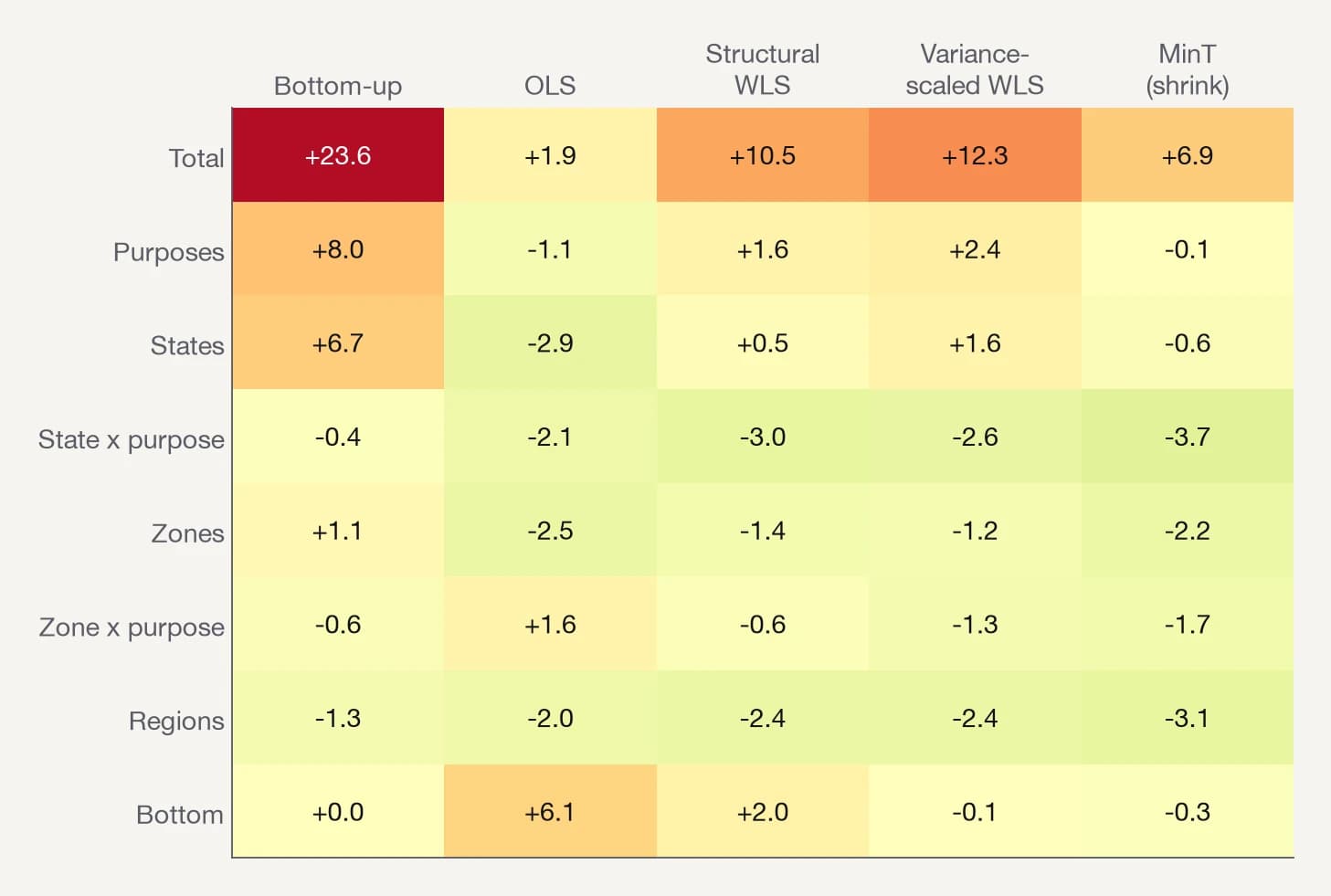
The grouped structure, the tourism data's region-and-purpose version of the retailer's store by product, favours MinT more, as Figure 5 shows. MinT improves the six intermediate levels and comes out 1.3% better than the base forecasts on average. The extra aggregates also hold the total closer to its own forecast, and its loss falls from 12% to 7%.

Bias at the national total

We also checked that the guarantee holds. In every fold, the OLS sum of squared errors over all 415 series is lower than the base forecasts' sum, as the theorem requires, while the total's own error rises. The same sum is higher for MinT in every fold, which does not contradict the theorem, whose guarantee for MinT is stated in its own weighted norm.

Bias is the reason the total loses, and the retailer shows why reconciliation cannot fix it. Suppose that in another month Portugal sells 200 units, Lisbon 120 and Porto 80, and that every forecast comes in 10% low: 180, 108 and 72. The three forecasts add up (108 + 72 = 180), so reconciliation has nothing to move, and the plan stays short at every level. Reconciliation redistributes a disagreement between levels, and a shortfall that every level shares is invisible to it.

Our base forecasts have exactly that kind of shortfall. Tourism grew after 2013 and ETS lags a trend, so the base forecasts are low at every level, by 4.4% at the total and by 6.7% at the bottom. The two biases differ, and MinT decides which one the reconciled total gets.

It gets most of the bottom's. In the last fold, MinT keeps only 0.11 of the total's own forecast and builds the rest from the states and the small series. Their 304 small residual variances add up to less than the total's one.

The reconciled total therefore moves most of the way to the bottom's larger bias, from −4.4% to −5.8%, and we find that the whole increase in its squared error is squared bias.

If bias is the cause, correcting it first should fix the total, and it does, as Figure 6 shows. Adding each series' mean in-sample residual moves nothing by as much as a percent, because ETS residuals average zero in sample.

Correcting each series by its mean error in the previous fold works, and that error is what a planner gets from the last backtest. We find that it turns MinT's total from 13% worse than the uncorrected base forecasts into 18% better than them. The correction is two lines, the previous fold's mean error per series added to the base forecasts before reconciling:

# e holds the previous fold's test actuals and base forecasts, one row per series and month
prev_err = (e["y"] - e["AutoETS"]).groupby(e["unique_id"]).mean()
Y_hat["AutoETS"] += Y_hat["unique_id"].map(prev_err).fillna(0.0).to_numpy()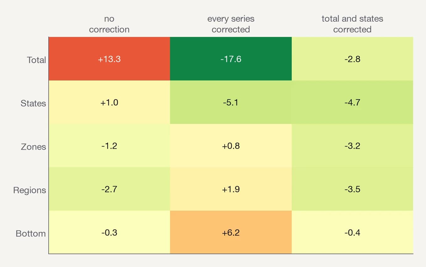

Nonetheless, the correction is noisy where the series are small, because 12 errors make a poor estimate of a bias, and it leaves everything below the states worse than before.

Correcting only the total and the seven states, where the bias can be estimated, improves every level against the forecast the planner had, the total by 3%. Against the corrected base forecast, a comparison Figure 6 does not show, the reconciled total is still 7.5% worse, because the bottom keeps its bias and the projection reconciles it back in.

Negative values and the weights

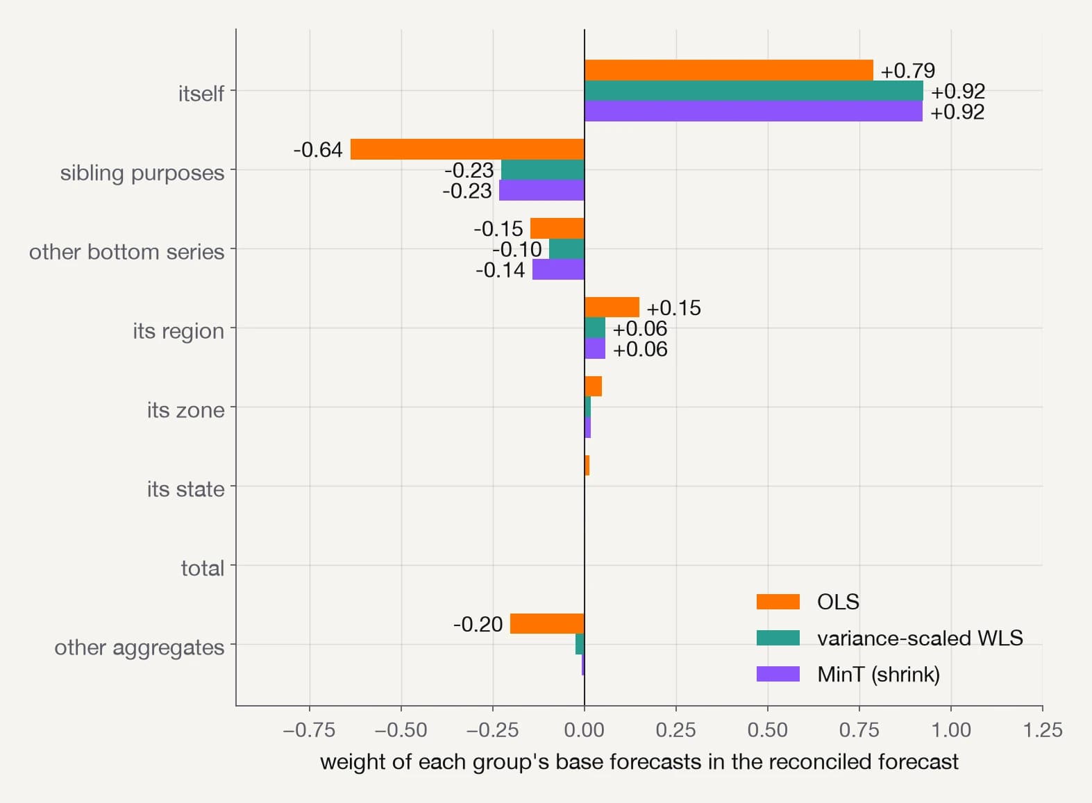
Negative reconciled values are a second cost we counted, and the weights explain them. We counted 33 negative monthly values in the base forecasts, 361 under OLS and 52 under MinT. Figure 7 shows where they come from: each reconciled forecast is a linear combination of every base forecast, with weights given by the rows of S P, and some of the weights are negative.

The recipes differ by method, and the difference is where the negatives come from. OLS subtracts a combined −0.64 of the three sibling purposes from one bottom series, while MinT keeps 0.92 of the series' own forecast and takes only −0.23 from the siblings. Wickramasuriya et al. [10] show how to add a non-negativity constraint, which intermittent retail series need more than tourism does.

Which series lose under MinT

The level means hide a wide spread, and the spread is where Prediction 1 lives. In Figure 8, we count the series-folds (one series in one fold) that got worse under MinT. The total loses in all four of its series-folds and the states in 57% of theirs. The share falls to a bit over a third at the zones and the regions, and it rises again to 47% at the bottom, where nearly half of the series-folds lose.

Repeat losers under MinT are the small ones. About a third of the 304 bottom series lose in at least three of the four folds, and they run far smaller than the series that rarely lose, a median of 17 thousand nights a month against 56 thousand.

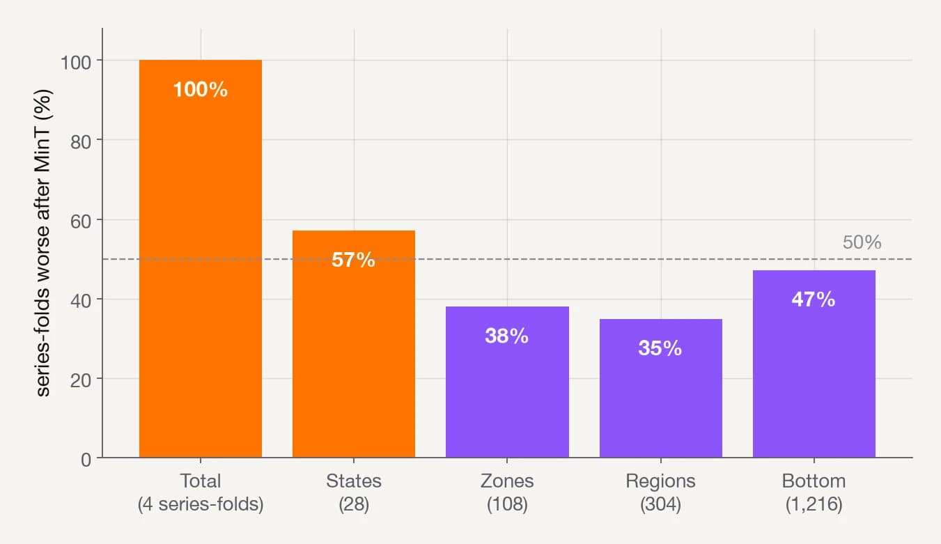
Prediction 1 holds after the fact: the fifth of bottom series with the best base forecasts in a fold lose 64% of the time and the fifth with the worst 39%. That test uses the realised error, so we also asked whether the losers can be identified in advance. They can, but only partly.

The best signal we found is the ratio, in the previous fold, of a series' out-of-sample RMSE to its in-sample residual standard deviation. A ratio below one means the residuals overstated the error, so W trusts the series less than it deserves and moves it further. Those are the series that lose, 61% of the time in the fifth with the lowest ratio against 42% in the fifth with the highest. Series size is a signal of similar strength.

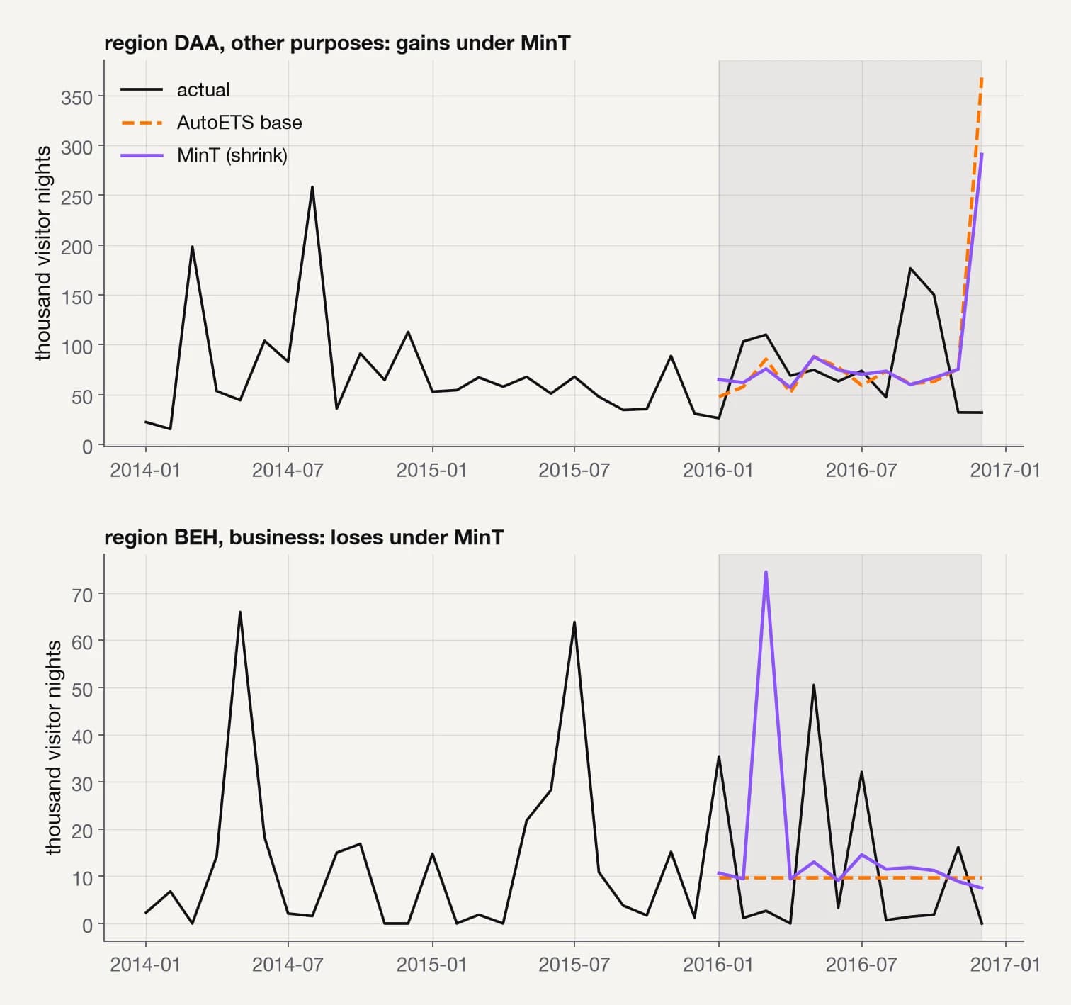
Figure 9 shows one series that gains under MinT in at least three folds, other-purpose travel in region DAA, and one that loses in at least three. The loser is business travel in region BEH, which averages ten thousand nights a month.

This loss has a mechanism. In March of the last fold, MinT gives it 74 thousand nights against an actual 3. The region's own base forecast has a spike that month, and the projection distributes the spike to the region's four purposes.

A foreign forecast at one level

In practice, the systems we meet rarely forecast every level with one model. A finance target replaces the total, or a supplier's numbers replace a region. We simulate this in two arms: the region forecasts are replaced with a seasonal naive forecast (noise, 26% worse in RMSSE at that level) or with the AutoETS forecast scaled by 0.85 (a bias, 14% worse).

Each arm is reconciled twice. In the aware run, W is re-estimated from the replacement model's residuals, so the weights know the level is worse. The blind run keeps the clean AutoETS residuals in W, which is what happens when a forecast arrives without its residuals:

region_ids = set(tags["Country/State/Zone/Region"])
mask = Y_hat["unique_id"].isin(region_ids)
Y_hat_bias = Y_hat.copy()
Y_hat_bias.loc[mask, "AutoETS"] = 0.85 * Y_hat_bias.loc[mask, "AutoETS"]

# blind: the reconciler still receives the clean in-sample fitted values
Y_rec_blind = hrec.reconcile(Y_hat_df=Y_hat_bias, Y_df=Y_fitted,
                             S_df=S_df, tags=tags)

# aware: the fitted values are scaled too, so the residuals reveal the change
Y_fitted_bias = Y_fitted.copy()
fmask = Y_fitted_bias["unique_id"].isin(region_ids)
Y_fitted_bias.loc[fmask, "AutoETS"] = 0.85 * Y_fitted_bias.loc[fmask, "AutoETS"]
Y_rec_aware = hrec.reconcile(Y_hat_df=Y_hat_bias, Y_df=Y_fitted_bias,
                             S_df=S_df, tags=tags)

Figure 10 shows both arms, and they move the other levels in different ways. Noise travels downward under OLS, which passes it to the small series and leaves the bottom 14.5% worse, because OLS weights every series equally in the raw units, so the large region forecasts dominate each small series' reconciled value. Variance-scaled WLS and MinT contain it, with the regions 2% worse in the aware run and 5% worse in the blind run.

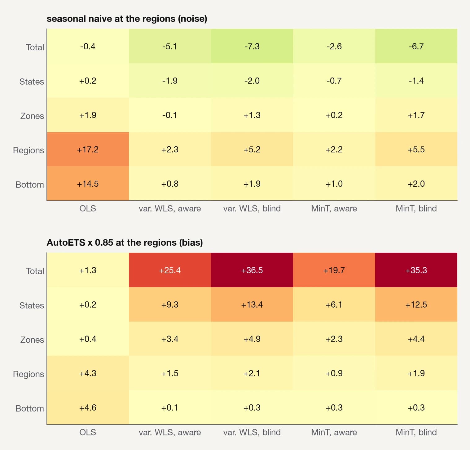
Prediction 2 held in its first half, since every level moved, and failed in its second, because the weights limit the damage even when they are blind to the change. Relative residual variances already carry the noise. What they cannot carry is a bias, as the second arm shows.

The noise arm also improves the total under the optimal family, by up to 7% for variance-scaled WLS, which surprised us until we checked the replacement's bias. Because the seasonal naive is less biased at the regions than ETS, the projection passes that upward, which is the third prediction showing up before its own experiment.

Our bias arm confirms it. A −15% bias at the regions makes the total 35% worse under MinT in the blind run and 20% worse in the aware run. Once the forecasts are coherent the errors add up as well, so the pooled bias is the same at every level, and it moves from −5.7% to −9.2%.

Nothing in W can see a bias, so the projection spreads it in proportion to the weights. The aware run does better only because scaling the fitted values also inflates the residual variance. Zero-shot forecasts are the case where a foreign forecast arrives at every level at once.

Reconciling Chronos-Bolt forecasts

Univariate foundation models such as Chronos forecast one series at a time and know nothing about hierarchies, so their forecasts are incoherent by construction. Nixtla's TimeGPT documentation reconciles forecasts of the quarterly tourism data: OLS gives a small gain in overall RMSE, and shrinkage weights give a loss, 14% at the total [11]. What we add is the size of the incoherence, the bias by level, and a control model on the same folds.

We use amazon/chronos-bolt-small [12], the successor of the Chronos model [13] we covered before, which forecasts all 415 series a year ahead in under a second on an Apple M4 Max laptop. Note that its forecasts are worse than AutoETS at the total (RMSSE 1.14 against 0.86) and equal at the bottom.

Our first problem was the point forecast. Chronos-Bolt predicts nine quantiles, and its predict_quantiles method returns the median as the "mean" (the source of chronos-forecasting 2.3.1 says so in a comment).

Medians of skewed series do not add up, in the way that the median income times the number of households is not the total income. Only the mean adds up, so we estimate it as the average of the nine quantiles and report both. The average is a trimmed mean that ignores the tails, so it still sits slightly low for a skewed series:

from chronos import BaseChronosPipeline
import torch

pipeline = BaseChronosPipeline.from_pretrained("amazon/chronos-bolt-small",
                                               device_map="cpu",
                                               torch_dtype=torch.float32)
ids = list(S_df["unique_id"])
QUANTILES = [0.1, 0.2, 0.3, 0.4, 0.5, 0.6, 0.7, 0.8, 0.9]

def chronos_forecast(history, start):
    history = history.sort_values(["unique_id", "ds"])
    context = [torch.tensor(history.loc[history.unique_id == uid, "y"].to_numpy(),
                            dtype=torch.float32) for uid in ids]
    quantiles, median = pipeline.predict_quantiles(
        context, prediction_length=HORIZON, quantile_levels=QUANTILES)
    mean = quantiles.numpy().mean(axis=-1)   # average of the nine quantiles
    dates = pd.date_range(start, periods=HORIZON, freq="MS")
    return pd.DataFrame({"unique_id": np.repeat(ids, HORIZON),
                         "ds": np.tile(dates, len(ids)),
                         "Chronos": mean.reshape(-1)})

Figure 11 measures how incoherent the raw forecasts are. For every aggregate, we compare its own forecast with the sum of its bottom-series forecasts, averaged over the horizon. With the mean forecast, we measure a median gap of about 5% at the total and about 6% at the levels below, against 1.6% to 4.8% for AutoETS at the total.

Using the medians instead doubles the gap, and in the last fold the 304 medians add up to 17% less than the forecast of the total.

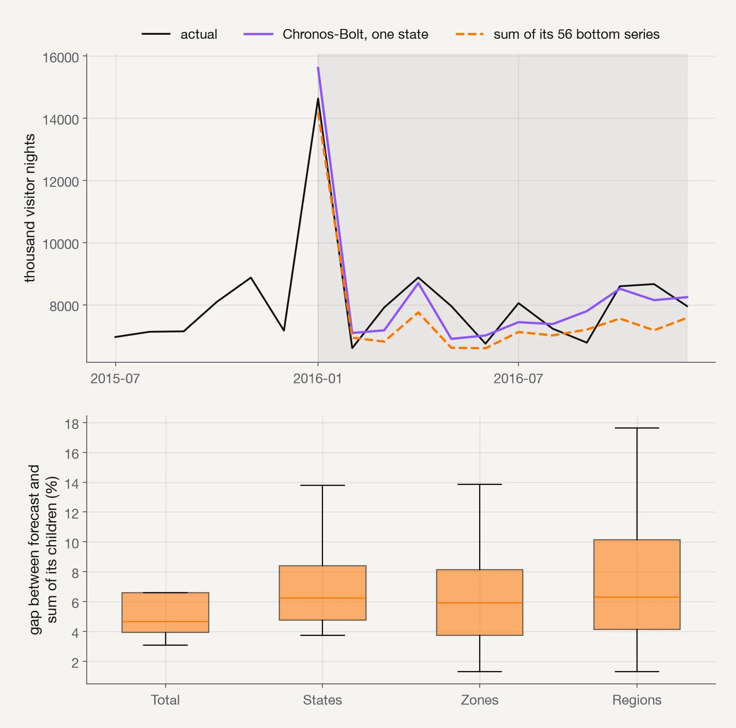
The top panel of Figure 12 shows why the medians fail: Chronos-Bolt under-forecasts the small series far more than the large ones. Its median is biased by −4.7% at the total and −15.8% at the bottom, where 85% of the series-folds are forecast too low.

Switching to the mean removes a third of that, leaving the bottom at −9.9% against −6.7% for AutoETS. The rest appears to be the zero-shot model pulling noisy series toward a flat, low level, and summing that many of them adds up a bias that no single series shows.

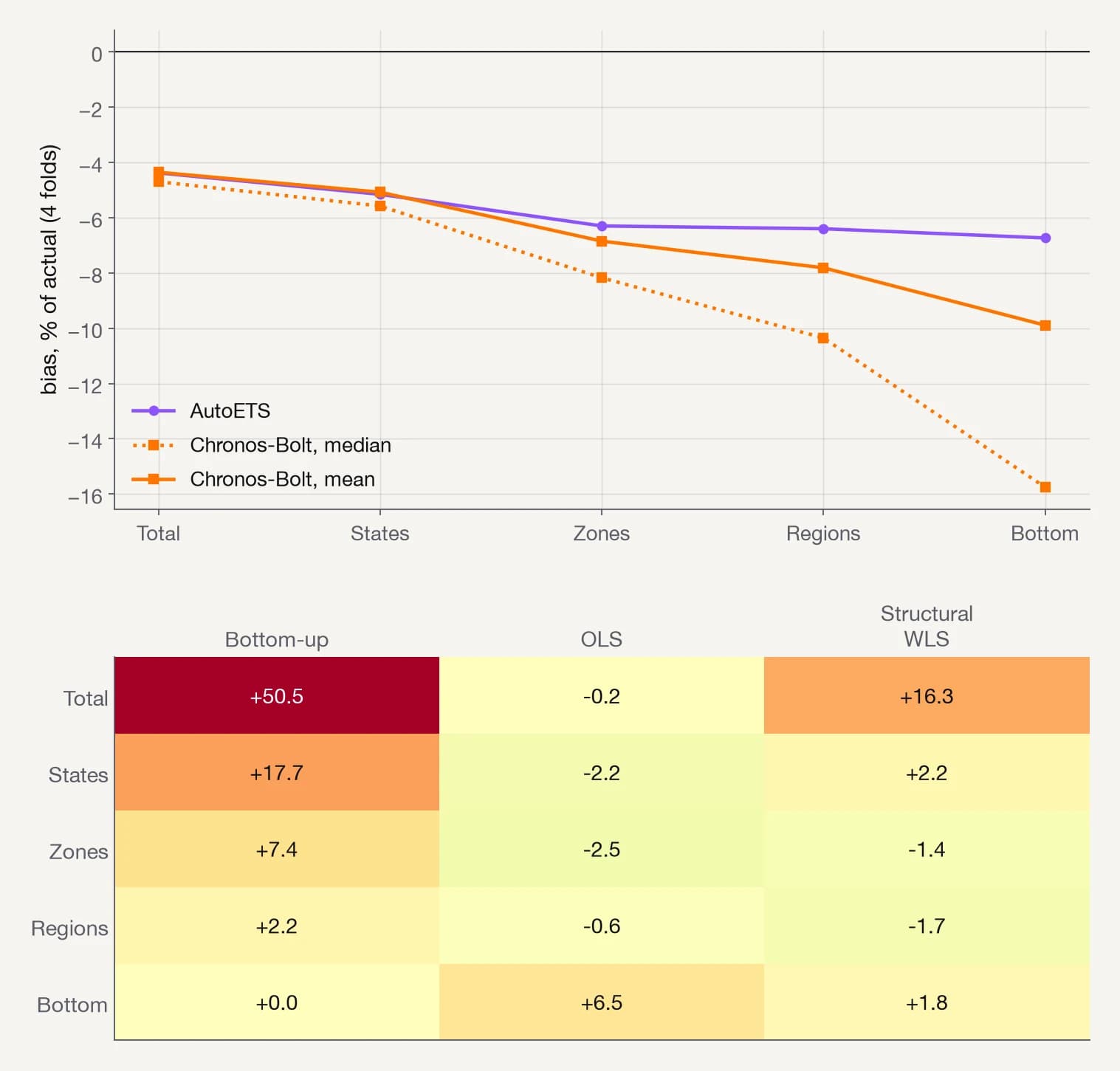
As shown in the bottom panel, reconciliation of the mean forecasts follows the pattern of Figure 10. Bottom-up, the simplest way to make foundation-model forecasts coherent, inherits the bottom's bias and makes the total 50% worse. Structural WLS, the choice when there are no residuals, still makes the total 16% worse. OLS is the only method that leaves the total alone while improving the middle levels, at the price of the bottom.

Even so, the reconciled Chronos-Bolt total remains 32% worse than the AutoETS base forecast. MinT needs residuals that a zero-shot model does not produce in sample.

With residuals from three 12-month backtests inside the training window, MinT makes the total 13% worse, close to the loss in the TimeGPT tutorial. We leave the like-for-like comparison, with rolling one-step residuals, to a follow-up.

Conclusion

On the monthly Australian tourism hierarchy, reconciliation does what the theory promises. The OLS sum of squared errors falls in every fold, and MinT is the most accurate method on average. Nevertheless, the national total gets 3% to 25% worse under MinT in every fold, and a third of the bottom series lose in at least three of the four folds. A biased level moves the bias of every other level, and zero-shot forecasts arrive with a bias that grows as the series get smaller.

Three of those four losses are bias, which W does not model, and the retailer says why: a shortfall that every level shares gives the projection nothing to move. The per-series losses are W itself, which moves a series by how noisy its residuals say it is rather than by how good its forecast was. We recommend the following before trusting a reconciled plan:

1. Measure the bias by level before reconciling and correct it where it can be estimated, at the aggregates, because the projection spreads whatever bias it is given.
2. Use MinT with shrinkage when the residuals come from the model that produced every level, and only the optimal family on a grouped structure such as store by product.
3. When a level is overridden, choose the weights by the override's likely error: OLS keeps a biased override's damage at and below its own level, while MinT or variance-scaled WLS, blind if necessary, contain a noisy one.
4. Use bottom-up only when the sum of the bottom forecasts agrees with the forecast of the total, and never with a quantile model's medians.

Two things we did not test are intermittent series, where zeros dominate and the non-negativity constraint of [10] matters, and hierarchies too young for a backtest, where the bias cannot yet be estimated. The experiment we leave open is to reconcile zero-shot forecasts with residuals from rolling one-step backtests, so that MinT meets a statistical model on equal terms.

References

[1] Hyndman, R. J., Ahmed, R. A., Athanasopoulos, G., & Shang, H. L. (2011). Optimal combination forecasts for hierarchical time series. Computational Statistics & Data Analysis, 55(9), 2579-2589. https://doi.org/10.1016/j.csda.2011.03.006

[2] Wickramasuriya, S. L., Athanasopoulos, G., & Hyndman, R. J. (2019). Optimal forecast reconciliation for hierarchical and grouped time series through trace minimization. Journal of the American Statistical Association, 114(526), 804-819. https://doi.org/10.1080/01621459.2018.1448825

[3] Hyndman, R. J., & Athanasopoulos, G. (2021). Forecasting: Principles and Practice (3rd ed.), Chapter 11, Forecasting hierarchical and grouped time series. OTexts. https://otexts.com/fpp3/hierarchical.html

[4] Panagiotelis, A., Athanasopoulos, G., Gamakumara, P., & Hyndman, R. J. (2021). Forecast reconciliation: A geometric view with new insights on bias correction. International Journal of Forecasting, 37(1), 343-359. https://doi.org/10.1016/j.ijforecast.2020.06.004

[5] Athanasopoulos, G., Ahmed, R. A., & Hyndman, R. J. (2009). Hierarchical forecasts for Australian domestic tourism. International Journal of Forecasting, 25(1), 146-166. https://doi.org/10.1016/j.ijforecast.2008.07.004

[6] Olivares, K. G., Garza, A., Luo, D., Challú, C., Mergenthaler, M., Ben Taieb, S., Wickramasuriya, S. L., & Dubrawski, A. (2022). HierarchicalForecast: A reference framework for hierarchical forecasting in Python. arXiv. https://arxiv.org/abs/2207.03517

[7] Hyndman, R. J., Lee, A. J., & Wang, E. (2016). Fast computation of reconciled forecasts for hierarchical and grouped time series. Computational Statistics & Data Analysis, 97, 16-32. https://doi.org/10.1016/j.csda.2015.11.007

[8] Athanasopoulos, G., Hyndman, R. J., Kourentzes, N., & Petropoulos, F. (2017). Forecasting with temporal hierarchies. European Journal of Operational Research, 262(1), 60-74. https://doi.org/10.1016/j.ejor.2017.02.046

[9] Schäfer, J., & Strimmer, K. (2005). A shrinkage approach to large-scale covariance matrix estimation and implications for functional genomics. Statistical Applications in Genetics and Molecular Biology, 4(1), Article 32. https://doi.org/10.2202/1544-6115.1175

[10] Wickramasuriya, S. L., Turlach, B. A., & Hyndman, R. J. (2020). Optimal non-negative forecast reconciliation. Statistics and Computing, 30(5), 1167-1182. https://doi.org/10.1007/s11222-020-09930-0

[11] Nixtla. Hierarchical forecasting with TimeGPT. TimeGPT documentation, accessed September 2026. https://www.nixtla.io/docs/forecasting/special-topics/hierarchical_forecasting

[12] Amazon (2024). Chronos-Bolt model card, amazon/chronos-bolt-small. Hugging Face. https://huggingface.co/amazon/chronos-bolt-small

[13] Ansari, A. F., Stella, L., Turkmen, C., Zhang, X., Mercado, P., Shen, H., Shchur, O., Rangapuram, S. S., Pineda Arango, S., Kapoor, S., Zschiegner, J., Maddix, D. C., Wang, H., Mahoney, M. W., Torkkola, K., Wilson, A. G., Bohlke-Schneider, M., & Wang, Y. (2024). Chronos: Learning the language of time series. Transactions on Machine Learning Research. https://arxiv.org/abs/2403.07815

All images are by the author unless noted otherwise.