Moirai: Time Series Foundation Models for Universal Forecasting

The future of predictive analytics: Explore Moirai, Salesforce’s new foundation model for advanced time series forecasting

This article was co-authored by Luís Roque and Rafael Guedes

Introduction

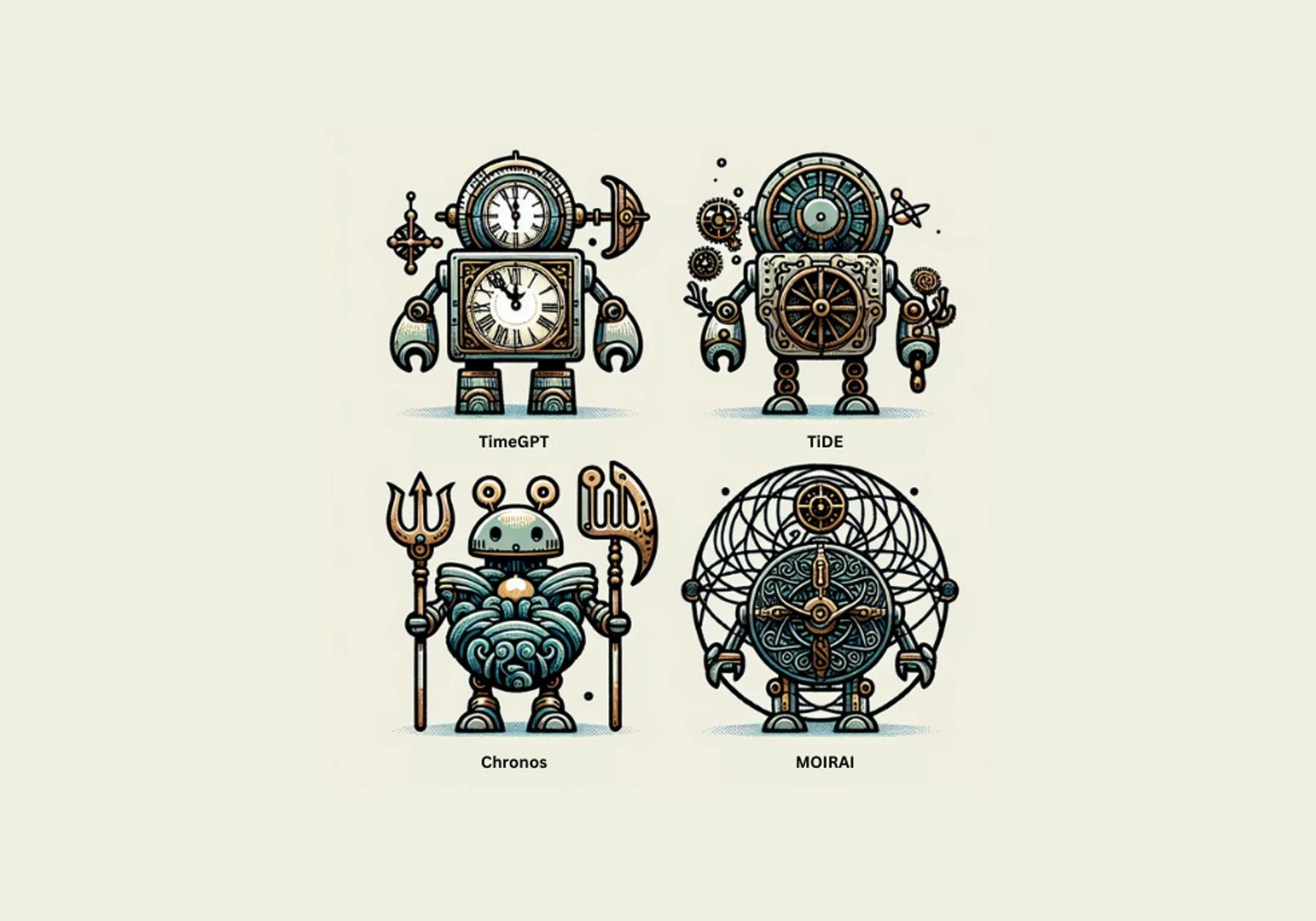
The development of time series foundation models has been accelerating over the last two quarters, and we have been witnessing the release of a new model nearly every month. It started with TimeGPT [1] in the last quarter of 2023, and since then, we saw the release of Lag-Llama [2], Google releasing TimesFM [3], Amazon releasing Chronos [4], and Salesforce releasing Moirai [5].

To understand the growing interest in foundation models, we should define their core capability: zero-shot inference. It refers to the ability to accurately perform tasks or make predictions on data that these models have never encountered during their training phase. This ability has been explored for models applied across various domains, such as natural language processing (NLP), computer vision, and multimodal tasks (combining text, images, etc.). The term “zero-shot” comes from the idea that the model sees “zero” examples from a specific task or data domain during training yet can “shoot” or aim at performing tasks in that area effectively. The term was introduced in the paper “Zero-Shot Learning with Semantic Output Codes,” authored by Hinton et al. and presented at the NIPS conference in 2009. Since then, it has emerged as one of the most prominent research topics and is now making its way into the field of time series analysis..

In this article, we explore Moirai, a new foundation model by Salesforce for time series forecasting. It builds on our series of articles about foundation models for time series forecasting, in which we provided detailed explanations and showcased the performance of models such as TimeGPT and Chronos on real-world datasets.

We provide an in-depth explanation of the architecture behind Moirai and the main components that allow the model to perform zero-shot inference. We also summarize the differences between the Moirai and the other two foundation models we have researched so far. We compare, for example, the size of the training data, the number of model parameters, and whether they allow multivariate forecasting.

Following this theoretical overview, we apply Moirai to a specific use case and dataset. We cover the practical implementation details and thoroughly analyze the model’s performance. Finally, we compare the performance of Moirai with TiDE and Chronos using a public dataset.

As always, the code is available on our GitHub.

Background

We define key concepts in time series forecasting to make it easier to understand the time series problems Moirai proposes to address.

Univariate time series forecasting focuses on predicting the future values of a single time series variable using only its past values. The forecasting model relies on the historical data of that single variable to identify patterns, trends, and cycles that can inform future predictions. An example would be forecasting tomorrow’s temperature based solely on past temperature records.

Multivariate time series forecasting involves predicting the future values of multiple related time series variables based on historical data. In this context, the forecast model accounts for the interdependencies and interactions between multiple variables to make predictions. For example, predicting the future sales of a product might consider not only past sales but also related factors such as marketing spend, seasonal trends, and competitor prices.

Covariates in time series forecasting are variables that can influence the outcome of the prediction. These variables can be known in advance or estimated for the forecast period. In both univariate and multivariate forecasting models, covariates incorporate additional insights beyond the historical data of the target variable. Examples include factors like holidays, special events, and economic indicators. Furthermore, in multivariate forecasting, covariates extend to include related time series data — these could be variables whose future values are either known or need to be predicted (see the example above).

Time series frequency refers to the intervals at which data points in a time series are recorded or observed, representing the regularity and granularity of the data over time. This frequency can range from high-frequency data, such as minute-by-minute transactions in financial markets, to low-frequency data, like annual economic indicators. Also, different frequencies can capture various trends, patterns, and seasonalities. For example, daily sales data may reveal patterns not visible in monthly aggregates, such as weekly cycles or the impact of specific days of the week.

Probabilistic forecasts extend beyond point predictions by providing a distribution of possible future outcomes. These output distributions represent the probability of different future values occurring, allowing for more informed decision-making under uncertainty. For instance, in scenarios where observations are strictly positive, such as sales volumes or energy consumption, probabilistic forecasts might use log-normal or gamma distributions to model the range of possible outcomes. Probabilistic forecasts are particularly useful in risk management and planning, as they enable stakeholders to evaluate the likelihood of various scenarios, from the most pessimistic to the most optimistic.

Moirai: the Time Series Foundation Model by Salesforce

Moirai is a foundational model for time series forecasting developed by Salesforce. It is designed as a universal model capable of predicting a wide range of time series. To achieve this flexibility, the model addresses several challenges associated with time series data, including the ability to:

• Handle all kinds of data frequencies (hourly, daily, weekly, etc);
• Accommodate any number and types of covariates, whether they are unknown in the future or known;
• Generate a probabilistic forecast using a flexible distribution that can be adapted to several cases.

The dataset is one of the core components of any foundation model. The authors built a large-scale and diverse dataset comprising 27 billion observations spanning nine distinct time series domains. Additionally, they introduced three main novel concepts: Multi Patch Size Projection Layers, Any-Variate Attention, and Mixture Distribution, each explained in detail in the following sections.

Multi Patch Size Projection Layers

Patching was first introduced to time series as PatchTST [7]. Its goal is to divide the time series data into patches of size P, which are shorter subsets of the original series. Then, why is patching useful in the context of foundation models in time series forecasting?

Time series forecasting aims to understand the correlation between data in each different time step. Foundation models tend to use an architecture based on transformers. While transformers work well for NLP applications, a single time step does not have semantic meaning like a word in a sentence. Hence, we need a way to extract local semantic information to apply the attention mechanism. Patching the series aggregates time steps into subseries-level components with richer semantic representations.

In simpler terms, we could say that as word embeddings represent words in a high-dimensional space, time series patches can be considered representations of segments of the series in a multidimensional space defined by their features.

This process brings numerous advantages, such as:

• Enabling the attention mechanism to extract local semantic meaning by looking into a group of time series instead of looking at a single time step;
• Reducing the number of tokens being fed to the encoder, consequently reducing the memory needed, allowing to feed longer input sequences to the model;
• With longer sequences, the model has more information to process and more meaningful temporal relationships to extract, potentially producing more accurate forecasts.

The patch size used by the authors depends on the data frequency, where lower frequency data has smaller patch sizes while higher frequency data has larger patch sizes:

• Yearly and Quarterly → Patch size 8
• Monthly → Patch size 8, 16, 32
• Weekly and Daily → Patch size 16, 32
• Hourly → Patch size 32, 64
• Minute-level → Patch size 32, 64, 128
• Second-level → Patch size 64, 128

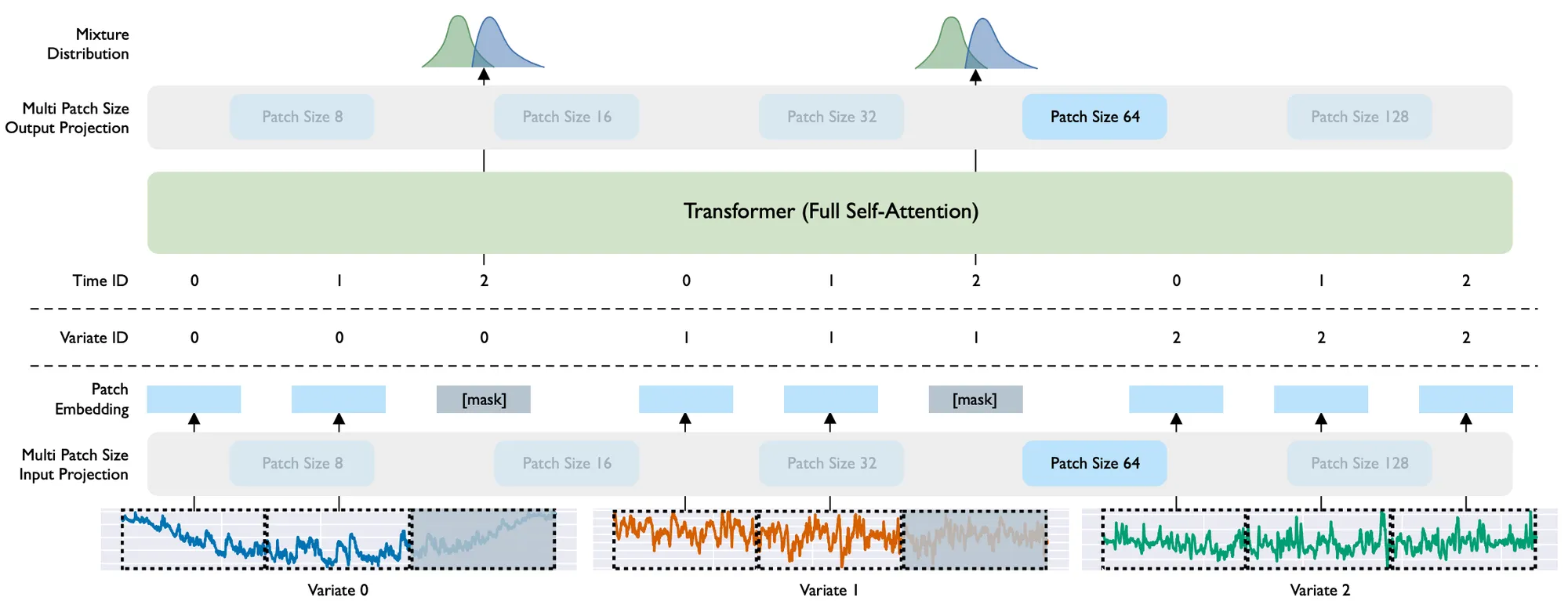
Regarding the model architecture, the authors used an input and output patch layer. After converting the data into patches, the input patch layer, a simple linear layer, maps the time series subset into a patch embedding to be fed to the encoder-only transformer layer. Later, a second patch layer is used to process the output of the encoder. The output tokens are then decoded via the multi-patch size output projection. Since there are five different patch sizes, the model has five different input patch layers and five different output patch layers activated according to the patch size used to process the input data.

To clarify further, let’s examine a specific example. Suppose we aim to forecast a quarterly time series. The data is segmented into P patches of size 8. These patches are subsequently processed by an input patch layer designed for patch size 8. The patch embeddings generated by this layer are then fed into an encoder-only Transformer, which processes the embeddings. Finally, the processed embeddings are output through a patch layer, again tailored for patch size 8.

Any-Variate Attention

The traditional Transformer architecture expects to receive a single sequence of target values. However, the model is expected to handle multiple sequences of target values and dynamic covariates in a multivariate time series scenario. Therefore, the authors introduced the Any-Variate Attention to allow Moirai to process multiple sequences.

The process starts by flattening the multiple time series (variates) into a single sequence of values. Then, a variate encoding is applied to allow the model to distinguish the different variates in the sequence, which is important when calculating the attention score.

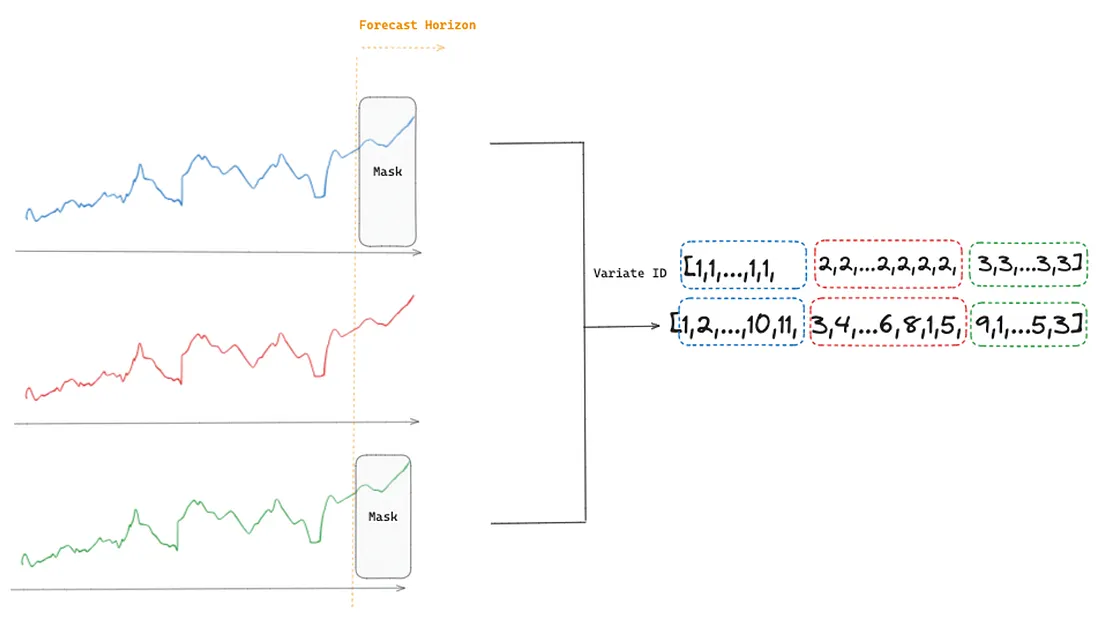
Any-Variate Attention has two fundamental characteristics: it achieves permutation equivariance with respect to variate ordering and permutation invariance with respect to variate indices.

Permutation equivariance regarding variate ordering means that if the sequence of observations within a variate is permuted, the model output for that variate reflects the same permutation. This property is required since we are working with time series, and the temporal dynamics must be preserved within each variate. Therefore, the model’s understanding of time series dynamics is consistent regardless of the input order.

Permutation invariance with respect to variate indices means that the model’s output does not change if the variates are reordered. For instance, let’s consider a scenario where we are processing temperature and humidity data as two variates in a multivariate time series setup. If we decide to swap the order in which these variates are presented to the model (first humidity, then temperature instead of first temperature, then humidity), it should not affect the final output. The model treats variate indices as interchangeable, focusing instead on the encoded relationships.

To achieve permutation equivariance/invariance, Moirai uses two distinct approaches:

• Rotary Positional Embeddings (RoPE) [8] ensures permutation equivariance by how its encoding works. It encodes the positional information by rotating the representation of tokens in the embedding space. The rotation angle is proportional to each token’s position in the sequence. Thus, it captures the absolute position of each token while maintaining the relative distances between any pair of tokens.
• Binary attention bias allows the model to be invariant — treating the variates as unordered. The model dynamically adjusts its focus by applying different attention biases (learnable scalars) based on whether elements belong to the same variate (m=n) or different variates (m≠n). This enables the Any-variate Attention mechanism to handle arbitrary numbers of variates and their permutations.

Mixture Distribution

Moirai is a probabilistic forecasting model, which means it learns the parameters of a distribution rather than merely providing a single point prediction. The output, being a distribution, enables decision-makers to evaluate the uncertainty of the predictions, as wider intervals indicate greater uncertainty from the model.

Like other probabilistic models such as DeepAR [9], the objective of Moirai is to estimate the parameters of a probability distribution by minimizing a loss function, specifically, the negative log-likelihood. There are several possible distributions for optimization. For instance, DeepAR can be configured to estimate the parameters of Gaussian, Beta, Negative Binomial, or Student’s t-distributions.

Since Moirai is a foundation model, it is designed to forecast various data domains and thus cannot be limited to a single distribution. To accommodate all possible scenarios, the model learns the parameters of a mixture of distributions, each suited to different kinds of data:

• Student's t-distribution is a robust option for most time series due to its ability to handle outliers and data with heavier tails.
• Negative Binomial distribution is useful for strictly positive count data, as it does not predict negative values.
• Log-Normal distribution effectively forecasts right-skewed data, such as economic indicators or natural phenomena. rictly positive count data, as it does not predict negative values.
• Low Variance Normal distribution is used for data clustered tightly around the mean and is suitable for high-confidence predictions.

TimeGPT vs Chronos vs Moirai: The Comparison

This section presents the similarities and dissimilarities between the foundation models we have studied in this and previous articles.

Table 1 compares the key characteristics of the foundation models. At this stage, we are not focused on comparing their performance, which will be covered in the next section. We should start by saying that Chronos and Moirai are open-source models and will benefit from community contributions. So, we recommend that in doubt, the selection should go for open-source models with greater community support and potential to improve over time. An important takeaway is that Chronos demonstrates much better data efficiency, requiring significantly less training data. Nonetheless, the model is not yet multivariate. Lastly, by looking at the number of parameters, we can see that time series models are considerably smaller than LLMs, making them more user-friendly and easier to deploy.

Moirai vs. Chronos: a comparison in a public dataset

In this section, we will use Moirai to forecast tourism visitors to Australia using a real-world dataset that is publicly available under the cc-by-4.0 license. Subsequently, we compare the forecasting performance of Moirai against Chronos (large version) and TiDE (to access the code that generated the forecast with Chronos and TiDE, please check our last article).

We enhanced the dataset with economic covariates (e.g., CPI, Inflation Rate, GDP) extracted from Trading Economics, which uses economic indicators based on official sources. We also perform some preprocessing to increase the usability of the dataset further. We stored the preprocessed dataset version here so that our experiments can be easily reproduced.

We start by importing the libraries and setting global variables. We set the date column, target column, dynamic covariates, the frequency of our series, and the forecast horizon.

%load_ext autoreload
%autoreload 2
import torch
import pandas as pd
import numpy as np
import utils
 
from datasets import load_dataset
from gluonts.dataset.pandas import PandasDataset
from huggingface_hub import hf_hub_download
 
from uni2ts.model.moirai import MoiraiForecast
 
TIME_COL = "Date"
TARGET = "visits"
DYNAMIC_COV = ['CPI', 'Inflation_Rate', 'GDP']
SEAS_COV=['month_1', 'month_2', 'month_3', 'month_4', 'month_5', 'month_6', 'month_7','month_8', 'month_9', 'month_10', 'month_11', 'month_12']
FORECAST_HORIZON = 8 # months
FREQ = "M"

 

After that, we load our dataset, which already has the exogenous features mentioned in the dataset description.

# load data and exogenous features
df = pd.DataFrame(load_dataset("zaai-ai/time_series_datasets", data_files={'train': 'data.csv'})['train']).drop(columns=['Unnamed: 0'])
df[TIME_COL] = pd.to_datetime(df[TIME_COL])
 
# one hot encode month
df['month'] = df[TIME_COL].dt.month
df = pd.get_dummies(df, columns=['month'], dtype=int)
 
print(f"Distinct number of time series: {len(df['unique_id'].unique())}")
df.head()

 

Distinct number of time series: 304

Once the dataset is loaded, we can split the data between train and test (we decided to use the last 8 months of data for our test set).

# 8 months to test
train = df[df[TIME_COL] <= (max(df[TIME_COL])-pd.DateOffset(months=FORECAST_HORIZON))]
test = df[df[TIME_COL] > (max(df[TIME_COL])-pd.DateOffset(months=FORECAST_HORIZON))]
 
print(f"Months for training: {len(train[TIME_COL].unique())} from {min(train[TIME_COL]).date()} to {max(train[TIME_COL]).date()}")
print(f"Months for testing: {len(test[TIME_COL].unique())} from {min(test[TIME_COL]).date()} to {max(test[TIME_COL]).date()}")

 

Months for training: 220 from 1998–01–01 to 2016–04–01

Months for testing: 8 from 2016–05–01 to 2016–12–01

Finally, we need to transform the pandas data frame into a GluonTS dataset to feed the model:

• We concatenate the training dataset (target and dynamic covariates) with only the dynamic covariates in the test set (the target in the forecast horizon will be null). We then replace the index of the pandas' data frame with the date column.
• We set the column that allows us to distinguish the different time series (unique_id).
• We defined which columns represent dynamic covariates known in the future (feat_dynamic_real).
• We define the target column (target) and the series frequency (freq).
• Note that there is no need to scale the data since the model handles it internally.

# create GluonTS dataset from pandas
ds = PandasDataset.from_long_dataframe(
    pd.concat([train, test[["unique_id", TIME_COL]+DYNAMIC_COV+SEAS_COV]]).set_index(TIME_COL), # concatenaation with test dynamic covaraiates
    item_id="unique_id",
    feat_dynamic_real=DYNAMIC_COV+SEAS_COV,
    target=TARGET,
    freq=FREQ
)

 

With the dataset ready, we can forecast using Moirai. For that, we need to load the model from Hugging Face and set the following parameters:

• prediction_length — which is the forecast horizon we defined earlier.
• context_length — how many items in the sequence the model can attend to (any positive integer).
• patch_size — the length of each patch. As seen previously, the authors set different patch sizes depending on the frequency. To use the pre-defined values, patch_size should be set to ‘auto’. It can also be set to any value from {auto, 8, 16, 32, 64, 128}.

# Prepare pre-trained model by downloading model weights from huggingface hub
model = MoiraiForecast.load_from_checkpoint(
    checkpoint_path=hf_hub_download(
        repo_id="Salesforce/moirai-R-large", filename="model.ckpt"
    ),
    prediction_length=FORECAST_HORIZON,
    context_length=24,
    patch_size='auto',
    num_samples=100,
    target_dim=1,
    feat_dynamic_real_dim=ds.num_feat_dynamic_real,
    past_feat_dynamic_real_dim=ds.num_past_feat_dynamic_real,
    map_location="cuda:0" if torch.cuda.is_available() else "cpu",
)
 
predictor = model.create_predictor(batch_size=32)
forecasts = predictor.predict(ds)
 
# convert forecast into pandas
forecast_df = utils.moirai_forecast_to_pandas(forecasts, test, FORECAST_HORIZON, TIME_COL)

 

Once the forecast has finished, we can plot the ground truth values and the predictions.

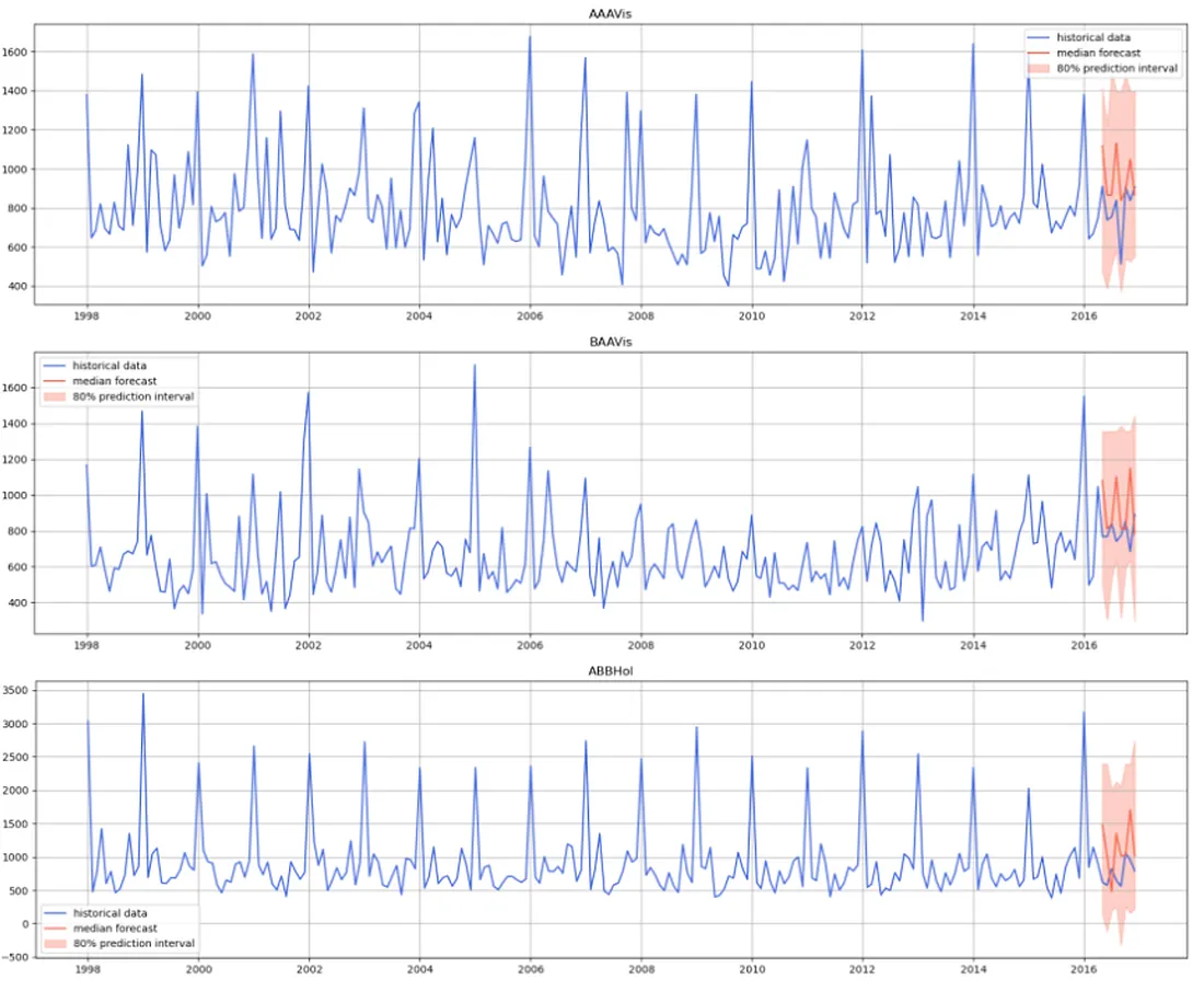
Figure 7 shows that Moirai struggled to forecast our time series and did not generate a stable forecast. Instead, it predicted several consecutive jumps with a higher magnitude than expected.

Having obtained the forecast from Moirai, we can now load the forecast generated by TiDE and Chronos and compute forecasting performance metrics for comparison. For better interpretability, we have used the Mean Absolute Percentage Error (MAPE) as our comparison metric.

As shown in Figure 8, Moirai has the highest MAPE in the entire forecast horizon. It slightly outperformed TiDE in one of the months but never managed to outperform Chronos. We conducted similar experiments on several private datasets, and the results consistently align with the findings presented in Figure 8. This consistency is relevant when analyzing foundation models, given that the training datasets are not publicly disclosed. It is plausible that any dataset from the public domain could have been used in their training data. In such circumstances, the model could have simply overfitted the training data.

Remember that Chronos does not allow the usage of covariates and assumes independence between the time series. This shows that the approach of Chronos is significantly better and has greater potential to be improved in the future.

Conclusion

In this article, we explored Moirai, one of the most recent foundation models for time series forecasting. This is one more example of a model capable of generating zero-shot inference. We have covered Chronos and TimeGPT in detail, and Moirai's approach and model architecture are quite different. Thus, we believe it carries scientific value and appreciate that it is open-source.

Our experiments indicate that Moirai was unable to outperform both TiDE and Chronos. In the case of TiDE, they have access to the same information, and TiDE was specifically trained on this data. However, when comparing Moirai’s performance with that of Chronos, we anticipated a more comparable or even superior performance from Moirai. This is because Moirai has the advantage of accessing external information through dynamic covariates and is a multivariate time series model capable of benefiting from cross-relationships between different series.

The AI race to develop foundational models for time series forecasting is just starting, and we will closely monitor its progress. Stay tuned.

About me

Serial entrepreneur and leader in the AI space. I develop AI products for businesses and invest in AI-focused startups. Founder @ ZAAI | LinkedIn | X/Twitter

References

[1] Garza, A., & Mergenthaler-Canseco, M. (2023). TimeGPT-1. arXiv. https://arxiv.org/abs/2310.03589

[2] Rasul, K., Ashok, A., Williams, A. R., Ghonia, H., Bhagwatkar, R., Khorasani, A., Darvishi Bayazi, M. J., Adamopoulos, G., Riachi, R., Hassen, N., Biloš, M., Garg, S., Schneider, A., Chapados, N., Drouin, A., Zantedeschi, V., Nevmyvaka, Y., & Rish, I. (2024). Lag-Llama: Towards Foundation Models for Probabilistic Time Series Forecasting. arXiv. https://arxiv.org/abs/2310.08278

[3] Das, A., Kong, W., Sen, R., & Zhou, Y. (2024). A decoder-only foundation model for time-series forecasting. arXiv. https://arxiv.org/abs/2310.106

[4] Ansari, A. F., Stella, L., Turkmen, C., Zhang, X., Mercado, P., Shen, H., Shchur, O., Rangapuram, S. S., Arango, S. P., Kapoor, S., Zschiegner, J., Maddix, D. C., Mahoney, M. W., Torkkola, K., Wilson, A. G., Bohlke-Schneider, M., & Wang, Y. (2024). Chronos: Learning the Language of Time Series. arXiv. https://arxiv.org/abs/2403.07815

[5] Woo, G., Liu, C., Kumar, A., Xiong, C., Savarese, S., & Sahoo, D. (2024). Unified Training of Universal Time Series Forecasting Transformers. arXiv. https://arxiv.org/abs/2402.02592

[6] Palatucci, M., Pomerleau, D., Hinton, G. E., & Mitchell, T. M. (2009). Zero-shot Learning with Semantic Output Codes. In Y. Bengio, D. Schuurmans, J. Lafferty, C. Williams, & A. Culotta (Eds.), Advances in Neural Information Processing Systems (Vol. 22). Curran Associates, Inc. Retrieved from https://proceedings.neurips.cc/paper_files/paper/2009/file/1543843a4723ed2ab08e18053ae6dc5b-Paper.pdf

[7] Yuqi Nie, Nam H. Nguyen, Phanwadee Sinthong, Jayant Kalagnanam. A Time Series is Worth 64 Words: Long-term Forecasting with Transformers. arXiv:2211.14730, 2022.

[8] Jianlin Su, Yu Lu, Shengfeng Pan, Ahmed Murtadha, Bo Wen, Yunfeng Liu. RoFormer: Enhanced Transformer with Rotary Position Embedding. arXiv:2104.09864, 2021.

[9] David Salinas, Valentin Flunkert, Jan Gasthaus. DeepAR: Probabilistic Forecasting with Autoregressive Recurrent Networks. arXiv:1704.04110, 2017.