MMM: Bayesian Framework for Marketing Mix Modeling and ROAS

Bayesian framework to model media channels performance, Return on Ad Spend (ROAS), and budget allocation using PyMC

This article was co-authored by Luís Roque and Rafael Guedes

Introduction

Scalable internet businesses depend on marketing to drive growth. Not only that, of course, but at a certain scale, very few companies can afford not to be extremely efficient in acquiring customers. Two hot topics that companies are investing heavily into bringing Artificial Intelligence (AI) capabilities into marketing are Media Mix Modeling (MMM) and Customer Lifetime Value (LTV) prediction. Both are focused on increasing the return on the investment organizations deploy on marketing. This article covers what MMM is and the best practices for applying it.

MMM is a technique that allows marketing teams to measure the impact of their investments and how they contribute to driving conversations. The complexity of this task has increased rapidly in the past years since the platforms available for advertising have skyrocketed. This phenomenon has spread potential customers over different media channels that we can separate into offline or online buckets. Traditional offline channels are unplugged from digital support and can range from the newspaper, radio, television ads, and coupons to a booth at a trade show. Online channels exploded, and companies use many of them together, such as email, social media, organic search, paid search, affiliate marketing, and influencer marketing.

One important caveat is that a good MMM requires an equally accurate data-driven attribution model, i.e., which channels contributed to acquiring a specific customer. Also, note that while attribution is performed at the user level, MMM is usually applied at the acquisition channel level. Data-driven attribution is out of the scope of this article.

In this article, our focus is twofold. First, we develop a Bayesian model designed to increase transparency on how each media channel performs. Secondly, we optimize the budget allocation to maximize our variable of interest, which in this case is revenue. Besides providing a detailed view of how a Bayesian approach works for MMM, we also give a walkthrough on implementing and applying it using a public dataset. We test the model accuracy and calculate each channel’s Return On Ad Spend (ROAS). Finally, we optimize a hypothetical budget across three channels to maximize revenue.

As always, the code is available on our GitHub.

Media Mix Modeling: What is it?

MMM empowers organizations across the globe by measuring the effectiveness of their advertising channels and providing transparency on how media spending impacts sales. These models play an important role in supporting the decision-making process of budget allocation across channels by optimizing a target variable of interest, such as sales, return on ad spend (ROAS), revenue, conversion, LTV, etc.

Over the past years, many studies have been performed, and several models have been proposed to try to model the influence that spending has on the variables of interest [1]. These models are based on weekly or monthly data aggregated geographically. We are interested in modeling the relationship between our dependent variables, one or many of the variables of interest defined above, and independent variables. Some independent variables are obvious, e.g., the ad spend across channels. Still, we can extend our approach to include further related effects from price, product distribution, inflation, weather, seasonality, and market competition.

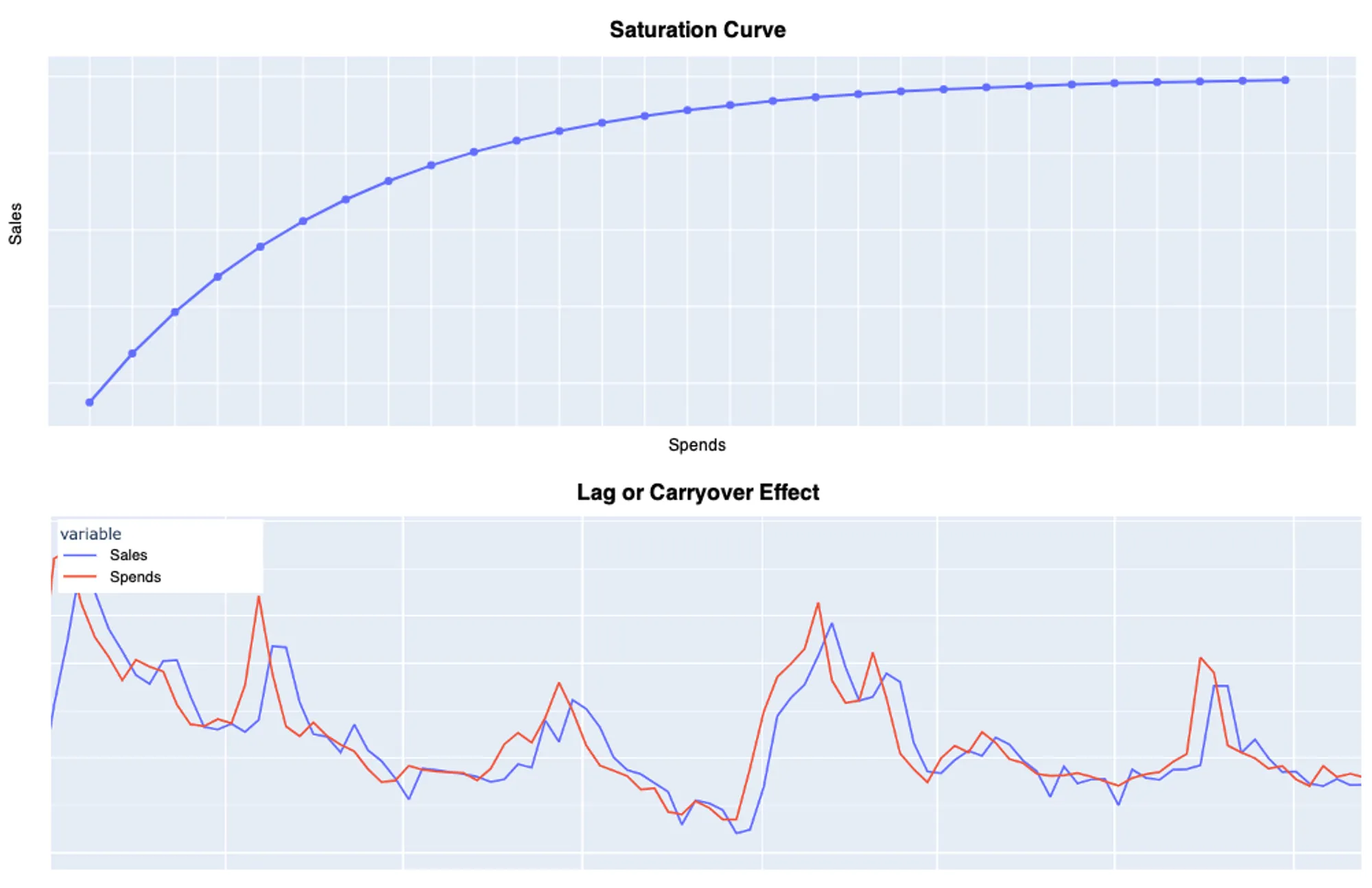
The traditional approaches rely on regression methods to infer causation from correlation. Nevertheless, the response of sales to media spending is not linear — there is saturation, which means diminishing returns at high-level spending. Moreover, advertisement has a lag or carryover effect, meaning spending in previous weeks can impact sales from the following weeks.

Bayesian Methods for Media Mix Modeling

Bayesian methods can be defined to consider the saturation/shape and lag/carryover effects.

Before diving into the model details, let’s define a hypothetical dataset for a better understanding of what variables the model takes. Suppose we have weekly data at a country level where each row represents a Week (t), and each column represents either a Media Channel (m) or a Control Variable (c) such as seasonality or product price. The media spend of channel m at week t is defined as Xt,m, and the control variable for the same week is defined as Zt,c.

Lag or Carryover Effect

The carryover effect is modeled by a function called adstock [1]. This function creates a cumulative effect of the spending in a specific channel. It transforms its time series through a weighted average of the media spend from the current week and previous L-1 weeks. L is the maximum duration of the carryover effect for a particular media channel, and it plays an important role in estimating the weight Wm in the weighted average equation.

L can be set differently across media channels. It is a hyperparameter to be defined by an expert. If no prior information exists for a particular channel, the authors advise setting L to a large number, such as 13, to capture potentially heavily lagged effects.

The equation that defines the weight can have two different forms:

1. Immediate/Geometric Adstock [2] when the advertisement effect peak happens at the same time as the ad exposure, i.e., we have a peak in sales in the same week we increased the spending of a media channel. In equation 2, αm is the retention rate of the ad effect.

2. Delayed Adstock [1] when the advertisement effect peak takes longer to build up and does not immediately impact sales. In equation 3, θm is the delay of the peak effect.

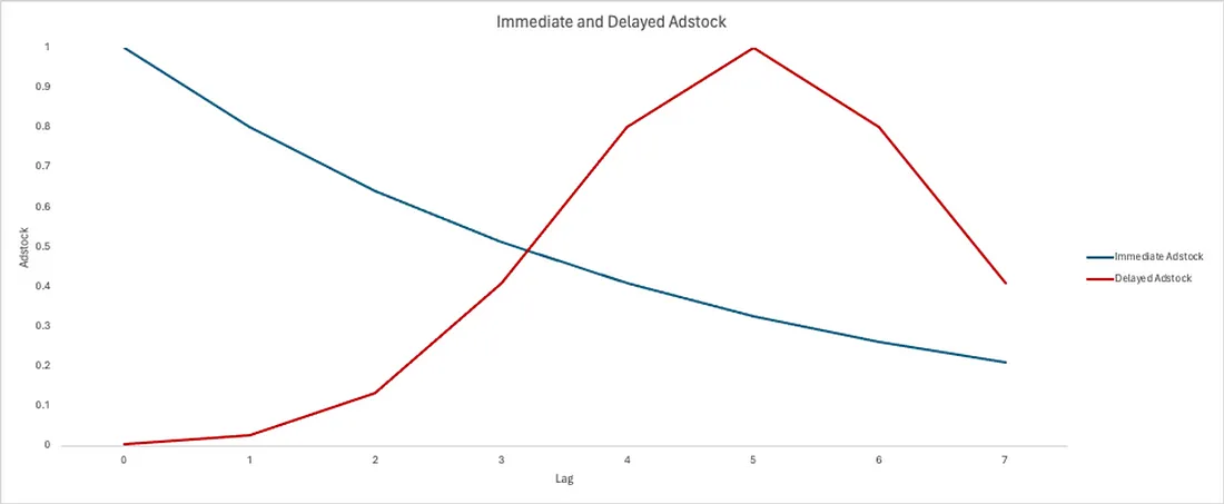
Let’s pick up our hypothetical dataset and calculate the Immediate and Delayed Adstock for the Facebook channel. To start, we added 5 more weeks to the dataset. We consider a retention rate (αm) of 80% and a peak delay (θm) of 5 weeks. After that, we calculate the weight for the immediate effect and the weight for the delayed effect to get to the final value of Immediate and Delayed Adstock at week 8.

Figure 3 shows how much each week’s spending contributes to the sales volume at week 8.

Saturation or Shape Effect

The saturation or shape effect is modeled by transforming the media spends through a curvature function such as the logistic saturation function [3]. It is defined as follows:

where x represents the media spends, and λ controls the steepness of the saturation curve, i.e., determines how quickly the media spend effect saturates. We can then interpret a low λ value as a more gradual increase in the response function, which translates into media spending having a noticeable effect over a large range of values. Conversely, higher λ values will result in diminishing returns on spending. Figure 4 shows these different behaviors very clearly.

It is difficult to know which parameters we should use for the model since these are quite specific for how each channel behaves. Nonetheless, in a Bayesian approach, these parameters are estimated using prior distributions. Hence, the model selects the most likely value parameters for given data. Therefore, we must set a distribution rather than a single value.

Combining the Carryover and Shape Effect

As mentioned in the previous two sections, to model the carryover and shape effect, we need to apply the transformations to the media spending of each channel. It raises the question of which transformation should be applied first. The authors suggest to:

• The shape effect follows the carryover if the media spending is heavily concentrated on certain periods.
• The carryover follows the shape effect if the media spending is evenly distributed across multiple time periods.

Since organizations usually tend to concentrate their marketing activity, the most common approach is the carryover → shape ffect combination.

That said, the dependent variable sales y at week t can be modeled through a linear combination of media spending and control variables. We also use a regression coefficient β to model different effects for different media channels.

where 𝛂 is the intercept. The function f(xm,t) encodes the contribution of media on the target variable considering adstock (carryover) and saturation effects. γc is the effect of control variable Zt,c and et is white noise.

Bayesian Model

The Bayesian approach begins with defining prior distributions for the model parameters, reflecting initial beliefs before considering the data. As new data is introduced, the likelihood function, which represents the probability of observing the data given the parameters, is calculated. In this context, the data includes media channels X and control variables Z, which explain the dependent variable y. Using Bayes theorem, the posterior distribution is obtained by combining the prior distributions and the likelihood function.

The authors rely on Gibbs Sampling [4] due to its sampling efficiency in selecting the parameter values for each media channel (X) and control variable (Z).

Remember that the model relies less on prior distributions to estimate the parameters when the data carries strong information and has clear patterns.

Nevertheless, the authors left some guidance on how to define prior distributions for each of the parameters:

• Retention rate (α) is constrained on [0, 1[ and should have a prior defined on [0, 1[ such as beta or uniform distribution.

br>

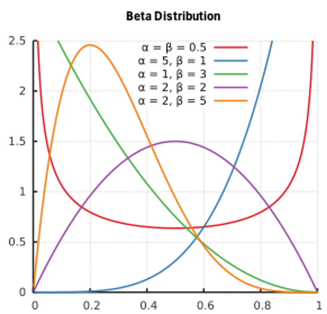
• Delay parameter (θ) is usually constrained on [0, L-1] and should have a prior such as uniform or scaled beta distribution.

br>

• Gamma (γ) and Intercept are usually modeled by a normal distribution.

br>

• Lambda (λ) is usually modeled by a gamma distribution.

br>

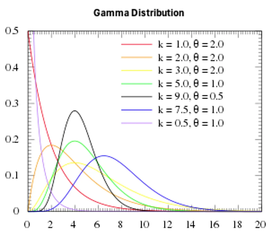
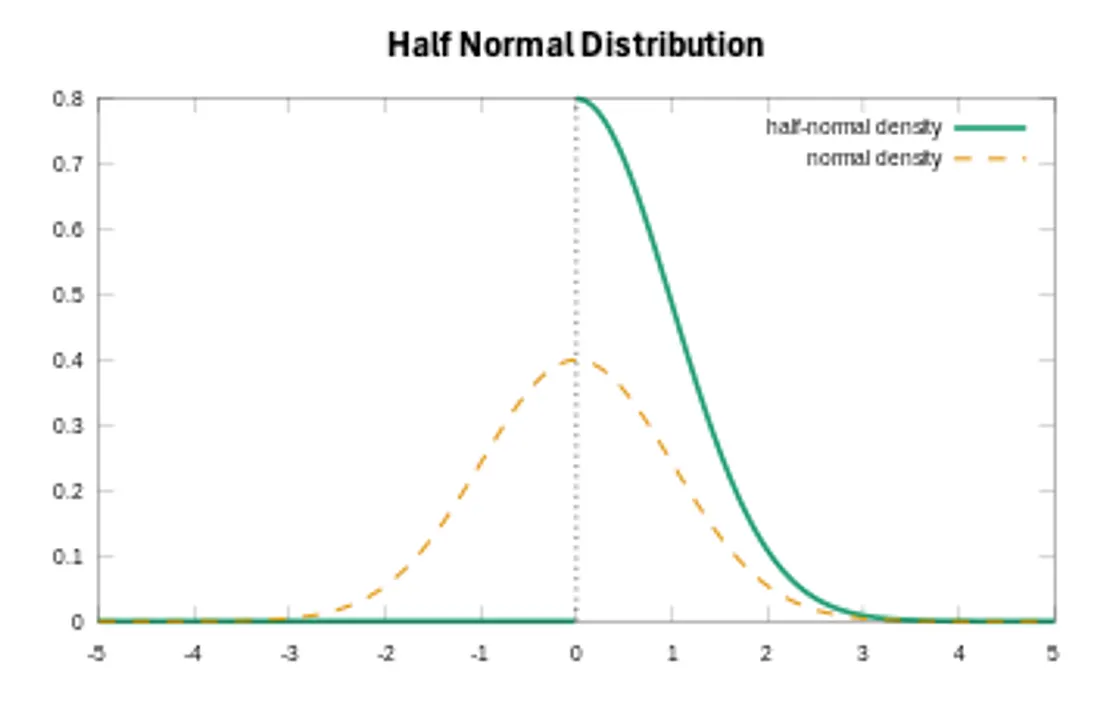
• Regression Coefficients (β) are usually modeled by nonnegative priors such as normal distribution since the media spending does not negatively affect y.

Bayesian Media Mix Modeling with PyMC

This section implements a Bayesian model on a public dataset from Kaggle under the License CC0: Public Domain. This dataset contains information about the spending on three different media channels (TV, Radio, and newspapers) and the sales for the same period.

The dataset is composed of the following:

• ID — identifies a row;
• TV Ad Budget ($) — advertisement spends on TV;
• Radio Ad Budget ($) —advertisement spends on Radio;
• Newspaper Ad Budget ($) — advertisement spends on Newspaper;
• Sales ($) — the target variable.

The fitted Bayesian model will help us calculate ROAS, retention, and saturation effect per channel. Besides that, it will also help us optimize the budget allocation for future weeks.

To estimate the reliability of the model, we will assess how well it can model the dependent variable on unseen data based on the spending of each media channel and control variables. We resort to regression metrics such as Mean Absolute Error (MAE). In terms of benchmarking, we use a naive model that always predicts the average value of the training data. By the way, companies often rely on this when no MMM is available.

We start by importing the libraries:

%matplotlib inline
%load_ext autoreload
%autoreload 2
import arviz as az
import datetime
import pandas as pd
import seaborn as sns
import matplotlib.pyplot as plt
import numpy as np
import utils
from pymc_marketing.mmm.delayed_saturated_mmm import DelayedSaturatedMMM
from sklearn.metrics import mean_absolute_error

 

Then, we load the dataset and perform some basic preprocessing tasks. We simplified the column names and added a new date column based on the ID. It helps enrich the dataset with control variables such as seasonality and trend.

# load data and rename columns
df = pd.read_csv('data/data.csv')
 
# create datetime column
df['ds'] = df['id'].apply(lambda x: pd.to_datetime("2024-02-26")-datetime.timedelta(weeks=len(df)-x))

 

After that, we perform some exploratory data analysis to understand correlations within the data:

1. We evaluate the correlation between the dependent variable and each media channel.

• TV is the most correlated feature with sales, while Newspaper is the least correlated.

corr_matrix = df[['sales', 'tv', 'radio', 'newspaper']].corr()
sns.heatmap(corr_matrix, annot=True, cmap='Blues')
plt.show()

 

2. We plot sales versus each media channel to assess if there is any lag effect between a peak in spending and a peak in sales:

• There is no clear trend or seasonality in sales.
• The effect of TV advertisements seem to have an immediate impact on sales.
• The effect of Radio advertisements also seem to have an immediate impact on sales. For example, in weeks 1, 2, and 3 in 2022, where TV had lower advertisement values, we see 2 spikes in sales, which match the spikes in Radio.
• The effect from Newspaper advertisements seem to have a 1-2 week lag, but it is hard to tell since TV and Radio advertisements ran simultaneously.

# only sales
utils.line_plot(df.copy(), ['sales'], 'Sales over Time')
 
# sales vs tv spends
utils.line_plot(df.copy(), ['sales', 'tv'], 'Sales vs TV over Time')
 
# sales vd radio spends
utils.line_plot(df.copy(), ['sales', 'radio'], 'Sales vs Radio over Time')
 
# sales vs newspaper spends
utils.line_plot(df.copy(), ['sales', 'newspaper'], 'Sales vs Newspaper over Time')

 

With the EDA finalized, we can start preparing the modeling part by:

1. Splitting the data into train and test:

train_df = df.sort_values(by='ds').iloc[:-5,:]
test_df = df.sort_values(by='ds').iloc[-5:,:]

 

2. Use the weekly data we generated before to extract control variables such as trend and seasonality.

We resort to the time series model Prophet from Meta to decompose our time series into trend and seasonality, and we use those as control variables.

seasonality, trend = utils.extract_trend_seasonality(train_df, 'sales', 5)
train_df.loc[:, 'seasonality'] = seasonality[:-5]
test_df.loc[:,'seasonality'] = seasonality[-5:]
train_df.loc[:,'trend'] = trend[:-5]
test_df.loc[:,'trend'] = trend[-5:]

 

3. Set the different hyperparameters for the model. These parameters can be defined through a traditional ML hyperparameter search. We optimize some regression metrics by changing the dist, mu, and sigma values. Remember that higher standard deviation values (sigma) give the model more freedom while searching for the optimal parameter.

my_model_config = {'intercept': {'dist': 'Normal', 'kwargs': {'mu': 0, 'sigma': 2}},
 'beta_channel': {'dist': 'HalfNormal', 'kwargs': {'sigma': 2}},
 'alpha': {'dist': 'Beta', 'kwargs': {'alpha': 1, 'beta': 3}},
 'lam': {'dist': 'Gamma', 'kwargs': {'alpha': 3, 'beta': 1}},
 'likelihood': {'dist': 'Normal',
  'kwargs': {'sigma': {'dist': 'HalfNormal', 'kwargs': {'sigma': 2}}}},
 'gamma_control': {'dist': 'Normal', 'kwargs': {'mu': 0, 'sigma': 2}},
 'gamma_fourier': {'dist': 'Laplace', 'kwargs': {'mu': 0, 'b': 1}}}

 

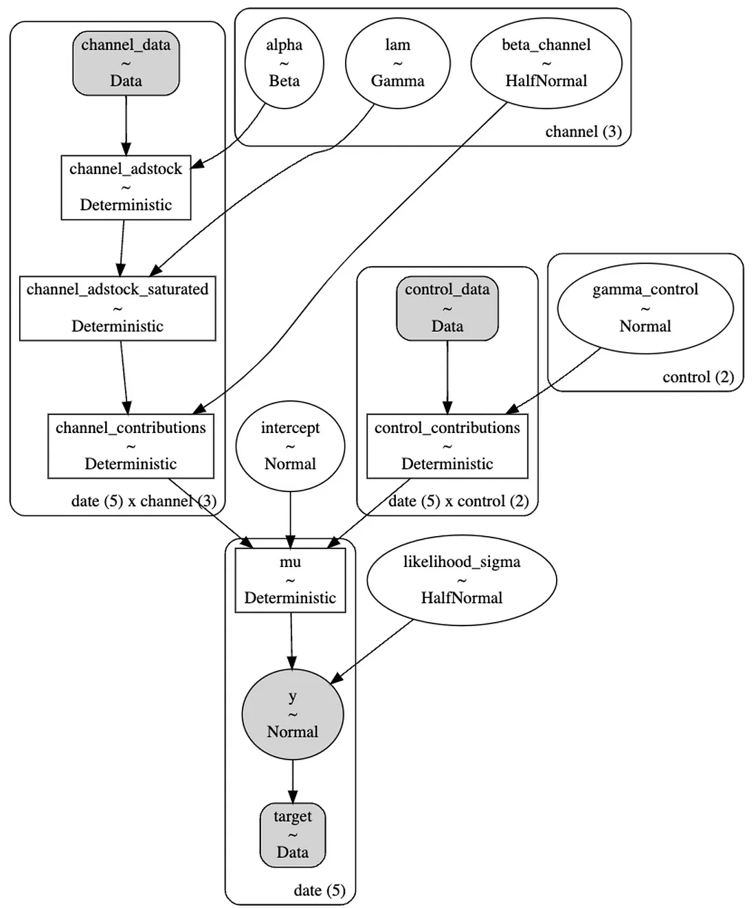
In Figure 13, we present the Kruschke diagram of the model we implemented. It provides a concise overview of the definitions we made earlier. There are a few aspects to consider when reading such a diagram. Note that we find the variables and their respective distributions within each node. For instance, the circle containing α depicts a beta distribution, as defined earlier. Shaded nodes represent the observed variables. Rounded-corner boxes indicate repetition. For example, since we have three acquisition channels, we set a distinct set of α, β, and λ parameters for each channel. The arrows illustrate dependencies. In our model, two arrows point to the likelihood function: one indicates a dependency on the mu parameter and another on the sigma parameter. The mu parameter itself has three additional dependencies. Recall that we chose to model sales by integrating the carryover effect, shape effect, and control variables.

Now that we have defined the training and testing sets and the model config, we can initiate the Bayesian model and fit it into the training data.

• Media Channels ["tv", "radio", "newspaper"]
• Control Variables ["seasonality", "trend"]
• From EDA, maximum adstock lag (delay parameter) does not seem higher than 2

mmm = DelayedSaturatedMMM(
    model_config=my_model_config,
    sampler_config={"progressbar": True},
    date_column="ds",
    channel_columns=["tv", "radio", "newspaper"],
    control_columns=["seasonality", "trend"],
    adstock_max_lag=2,
)

mmm.fit(X=train_df[['ds', 'tv', 'radio', "newspaper", "seasonality", "trend"]], y=train_df['sales'], target_accept=0.95, chains=4, random_seed=42)

After fitting the model, we can check how well it fits the training data by comparing the sampling predictions (blue) and the true values (black). In our case, they are well aligned.

mmm.sample_posterior_predictive(train_df[['ds', 'tv', 'radio', "newspaper", "seasonality", "trend"]], extend_idata=True, combined=True)
mmm.plot_posterior_predictive(original_scale=True);

Now, we can start interpreting the model using several approaches:

1. Checking the parameter estimation:

• Radio seems to have the most return on investment since its coefficient (beta) is the highest (1.185), followed by TV and Newspaper.
• The retention rate α is 3.2% for TV, 2.3% for Radio and 23.9% for Newspaper.

az.summary(data=mmm.fit_result,
    var_names=[
        "intercept",
        "likelihood_sigma",
        "beta_channel",
        "alpha",
        "lam",
        "gamma_control",
    ],
)

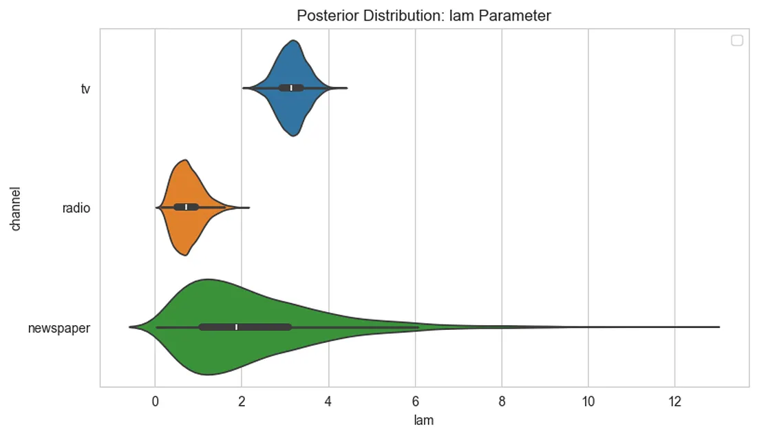
• The saturation rate λ is higher on TV (3.138), which accounts for 73% of the total spending. In Figure 12, we can more easily compare the saturation rate for the 3 channels.

2. Checking channel contribution and ROAS:

• ROAS is calculated by setting the spend of one of the media channels to zero to assess what happens to the predicted sales compared to the current sales. For example, if we set the media spend of Newspaper to zero, we are not expecting a big decline in sales. Therefore, its ROAS will be low.
• Although TV has the highest contribution because it had higher spending, we can see that the model predicts a higher ROAS for Radio.

# channel contribution
fig = mmm.plot_channel_contribution_share_hdi(figsize=(7, 5))

# ROAS calculation
utils.plot_ROAS(mmm, train_df, ["tv", "radio", "newspaper"])

3. Finally, we can also assess what would happen if we increase in 50% the advertisement spend in each channel by taking into consideration the carryover and saturation effect.

X axis is the input channel data percentage level:

• When =1, we have the model input spend data.
• When =1.5, we have how much the contribution would have been if we had increased the spending by 50%.

Newspaper seems to have reached its saturation point since a 50% increase in spending would not bring much more contribution.

Radio seems much less saturated than TV based on the slope of both lines.

plt.rcParams["figure.figsize"] = (20,5)
mmm.plot_channel_contributions_grid(start=0, stop=1.5, num=12);

To understand if our conclusions are valid, we can use our test set to assess the ability of our model to predict future sales based on the media channels and control variables. For that, we use MAE and compare it with a naive model.

• We had an MAE of 2.01 for a target average of 13.8.
• We have an error 58% lower than the baseline.

y_out_of_sample = mmm.sample_posterior_predictive(X_pred=test_df[['ds', 'tv', 'radio', "newspaper", "seasonality", "trend"]], extend_idata=False)
y_pred = [np.median(x) for x in y_out_of_sample['y']]

print(f"MAE: {mean_absolute_error(test_df['sales'], y_pred)} for an average target of {test_df['sales'].mean()}")
print(f"MASE: {mean_absolute_error(test_df['sales'], y_pred)/mean_absolute_error(test_df['sales'], [train_df['sales'].mean()]*5)}")

MAE: 2.008733107943637 for an average target of 13.8 MASE: 0.41701581608539257

The regression results show that the model is reliable and does a good job of modeling sales based on the media channels and control variables.

Budget Allocation

Since we assume that the effect of spending on sales is not linear, it will saturate at some point. Therefore, we need to determine which saturation function better fits our data. We have two function options to model saturation:

• A sigmoid function where α (alpha) is the saturation point, which means an increase in spending will not increase sales, and λ (lambda) influences the slope of the curve, where higher values make the curve steeper.

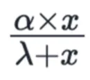
• Michaelis-Menten function where α (alpha) is the maximum contribution a channel can have and λ (lambda) is the moment when the curve adjusts its direction, i.e., the slope.

To determine which curve will suit our data better, we will use our fitted MMM to calculate the parameters for each function. After that, we plot both of them and visually check which one performs a better fit.

• For our specific use case, the sigmoid function performed better.

# plot and extracting alpha and lambda
sigmoid_response_curve_fig = mmm.plot_direct_contribution_curves(show_fit=True)
sigmoid_params = mmm.compute_channel_curve_optimization_parameters_original_scale(method='sigmoid')

mm_response_curve_fig = mmm.plot_direct_contribution_curves(show_fit = True, method='michaelis-menten')
mm_params = mmm.compute_channel_curve_optimization_parameters_original_scale(method='michaelis-menten')

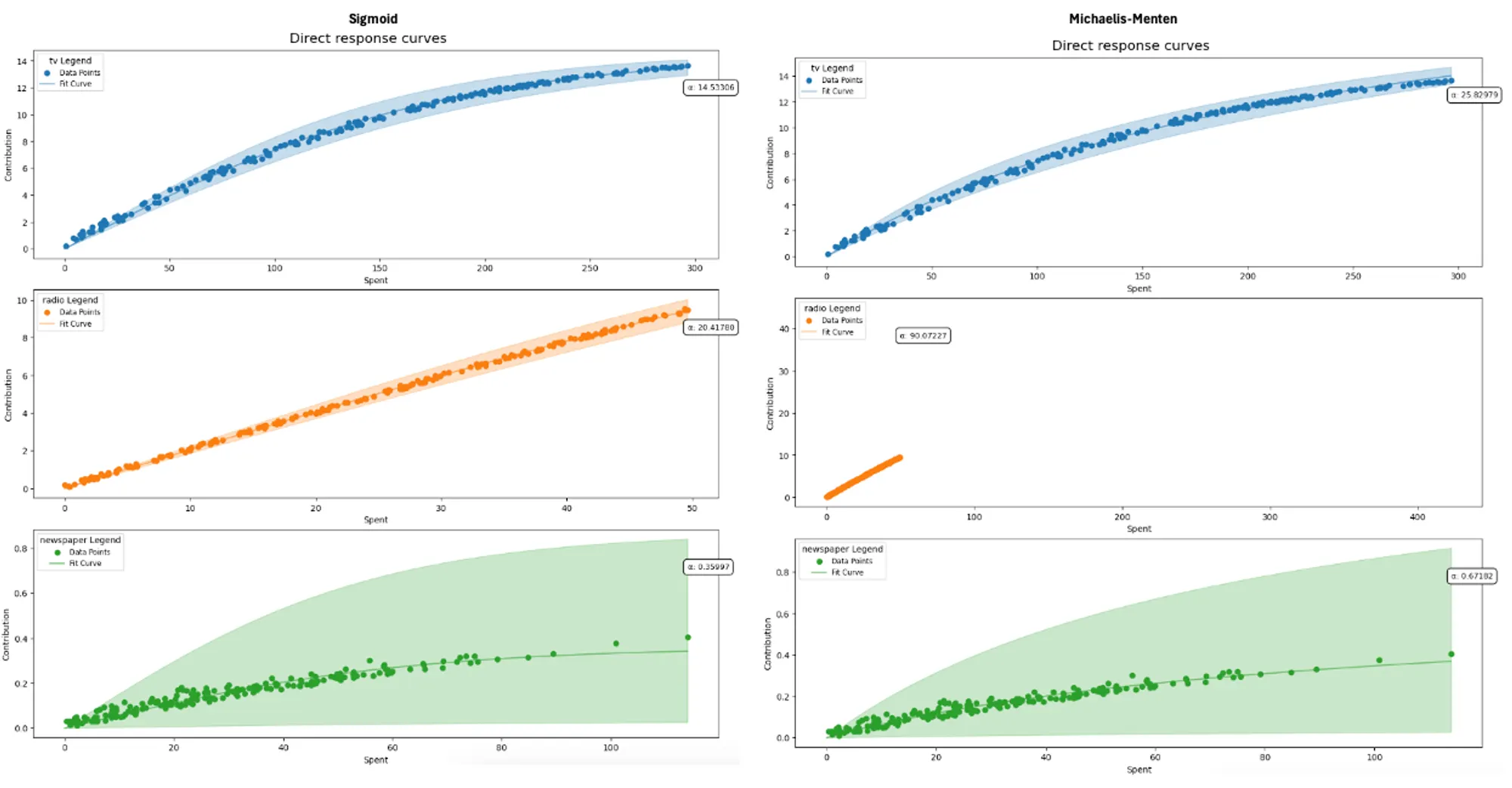
Now that we have each media channel’s sigmoid parameters (α and λ), we know the saturation point of each channel. Thus, additional spending will not increase the returns, while the amount invested in another channel can have that desired effect.

We can use an algorithm to optimize the budget allocation based on the channel saturation, the total budget available, and the budget constraints for each channel. PyMC has an implementation of Sequential Least Squares Quadratic Programming (SLSQP). It maximizes the total contribution from all channels, taking into consideration all of those three variables:

• The total budget limitation;
• The minimum and maximum spending limits for each channel;
• The saturation curve.

result_sigmoid = mmm.optimize_channel_budget_for_maximum_contribution(
    method = 'sigmoid', #define saturation function
    total_budget = 500, # total budget
    parameters = sigmoid_params, # sigmoid parameters extracted previously
    budget_bounds = {'tv': [75, 296], 'radio': [10, 300], 'newspaper': [1, 25]} # budget constraints by channel
)

Table 4 shows the results of our budget allocation, where Radio is the channel with the highest estimated contribution, and TV is the channel where we are advised to spend the highest budget.

Budget allocation under market uncertainty

In the current economy, we are facing a lot of uncertainty. Thus, we must design a budget allocation strategy that accommodates various scenarios.

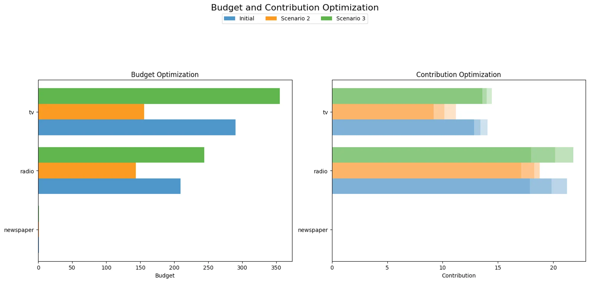
Let’s consider three different scenarios:

• Initial: the economy stays stable, and the budget allocation is the same as calculated in the previous section.
• Scenario 2: the economy goes through a recession period, and our budget is cut by 40%
• Scenario 3: the economy gets more favorable and starts growing, and our budget increases by 20%

We will use the same fitted MMM model and the same sigmoid parameters of the model to optimize the budget allocation under these different scenarios. We will use the same code as before, but we loop over the different scenarios to reduce or increase the available budget this time.

scenarios_result = []
total_budget = 500
channels = ['tv', 'radio', 'newspaper']
 
for scenario in np.array([0.6, 1.2]):
    scenarios_result.append(
        mmm.optimize_channel_budget_for_maximum_contribution(
            method="sigmoid",  # define saturation function
            total_budget=total_budget * scenario,
            parameters=sigmoid_params,
            budget_bounds={
                channel: [1, total_budget * scenario] for channel in channels
            },
        ).to_dict()
    )
_ = mmm.plot_budget_scenearios(
    base_data=result_sigmoid, method="sigmoid", scenarios_data=scenarios_result
)

 

As shown in Figure 19, under a recession scenario, the budget allocated to TV decreases significantly more than Radio compared to the initial scenario. This is expected because Radio has a higher ROAS, as we saw before. On the other hand, the budget allocated to TV and Radio increases similarly under a growth scenario.

Conclusion

AI for Media Mix Modeling can be the difference between getting a positive return on investment and acquiring valuable and loyal customers or draining our financial resources in the wrong media channel with the wrong customers.

In this article, we developed a Bayesian framework for Marketing Mix Modeling that can provide transparency and assess further potential for each company’s media channel to acquire new customers. In our approach, domain knowledge from the marketing teams can be incorporated by setting prior distributions. It contributes to improving the ability of the model to understand the relationship between the media channels and the dependent variable of interest (e.g., sales). Finally, the budget allocation strategy can be optimized depending on the capacity of the company to invest in acquiring new customers. In today’s macroeconomic scenarios, companies might be turning to profitability and, thus, reduce the available budget to invest in growth. We showed how to make a data-driven decision about where to cut with minimal impact. Conversely, we show where to invest if the scenario is more positive and the company wants to deploy more resources to grow faster.

We are currently developing and deploying new AI applications across organizations. For example, we are enhancing customer experience with generative AI and improving the planning process with time series forecasting. In this case, we demonstrate how AI can improve the efficiency of the marketing budget. From our experience, an advanced and mature organization in terms of AI adoption needs a suite of specialized AI models focused on its core activities.

About me

Serial entrepreneur and leader in the AI space. I develop AI products for businesses and invest in AI-focused startups. Founder @ ZAAI | LinkedIn | X/Twitter

References

[1] Yuxue Jin, Yueqing Wang, Yunting Sun, David Chan, Jim Koehler. (2017). Bayesian Methods for Media Mix Modeling with Carryover and Shape Effects.

[2] Dominique M. Hanssens , Leonard J. Parsons , Randall L. Schultz. (2003). Market response models: econometric and time series analysis. Springer Science & Business Media.

[3] Hill, A. V. (1910). The possible effects of the aggregation of the molecules of haemoglobin on its dissociation curves. Journal of Physiology, 40 (suppl), iv–vii. doi:10.1113/jphysiol.1910. sp001386.

[4] Gelfand, A. E. & Smith, A. F. (1990). Sampling-based approaches to calculating marginal densities. Journal of the American statistical association, 85 (410), 398–409

All images are by the authors unless noted otherwise.