Exploring the intricacies of encoder, multi-head attention, and positional encoding in large language models
This article was co-authored by Luís Roque and Rafael Guedes
Introduction
“You shall know a word by the company it keeps”
So, the semantic representation of a word is determined by the context in which it is being used. It is precisely in attendance to this assumption that the paper “Attention is all you need” by Ashish Vaswani et. al. [1] assumes its groundbreaking relevance. It set the transformer architecture as the core of many of the rapidly growing tools like BERT, GPT4, Llama, etc.
In this article, we examine the key mathematical operations at the heart of the encoder segment in the transformer architecture.
As always, the code is available on our GitHub.
Tokenization, Embeddings, and Vector Spaces
The first task one has to face while dealing with NLP problems is how to encode the information contained in a sentence so that the machine can handle it. Machines can only work with numbers which means that the words, their meanings, punctuation, etc, must be translated into a numeric representation. This is essentially the problem of embedding.
Before diving into what embeddings are, we need to take an intermediate step and discuss tokenization. Here, the blocks of words or pieces of words are defined as the basic building blocks (so-called tokens) which will lately be represented as numbers. One important note is that we cannot characterize a word or piece of word with a single number and, thus, we use lists of numbers (vectors). It gives us a much bigger representation power.
How are they constructed? In which space do they live? The original paper works with vector representations of the tokens of dimension 512. Here we are going to use the simplest way to represent a set of words as vectors. If we have a sentence composed of 3 words ‘Today is sunday’, each word in the sentence is going to be represented by a vector. The simplest form, and considering just these 3 words, is a 3-dimensional vector space. For instance, the vectors could be assigned to each word following a one-hot encoding rule:
‘Today’ — (1,0,0)
‘is’ — (0,1,0)
‘sunday’ — (0,0,1)
This structure (of 3 3-dimensional vectors), although possible to use, has its shortcomings. First, it embeds the words in a way that every one of them is orthogonal to any other. This means that one cannot assign the concept of semantic relation between words. The inner product between the associated vectors would always be zero.
Second, this particular structure could further be used to represent any other sentence of 3 different words. The problem arises when trying to represent different sentences made up of three words each. For a 3-dimensional space, you can only have 3 linearly independent vectors. Linear independence means that no vector in the set can be formed by a linear combination of the others. In the context of one-hot encoding, each vector is already linearly independent. Thus, the total amount of words the proposed embedding can handle is the same as the total dimension of the vector space.
The average amount of words a fluent English speaker knows is around 30k, which would mean that we need vectors of this size to work with any typical text. Such a high-dimensional space poses challenges, particularly in terms of memory. Recall that each vector would have only one non-zero component, which would lead to a very inefficient use of memory and computational resources.
Nevertheless, let’s stick to it to complete our example. In order to describe at least one simple variation of this sentence, we need to extend the size of our vectors. In this case, let’s allow the usage of ‘sunday’ or ‘saturday’. Now, every word is described by a 4-dimensional vector space:
‘Today’ — (1,0,0,0)
‘is’ — (0,1,0,0)
‘sunday’ — (0,0,1,0)
‘saturday’ — (0,0,0,1)
The 3 words in our sentence can be stacked together to form a matrix X with 3 lines and 4 columns:

import numpy as np
from scipy.special import softmax
import math
sentence = “Today is sunday”
vocabulary = [‘Today’, ‘is’, ‘sunday’, ‘saturday’]
# Initial Embedding (one-hot encoding):
x_1 = [1,0,0,0] # Today
x_2 = [0,1,0,0] # is
x_3 = [0,0,1,0] # Sunday
x_4 = [0,0,0,1] # Saturday
X_example = np.stack([x_1, x_2, x_3], axis=0)
The Single-Head Attention Layer: Query, Key, and Value
From X the transformer architecture begins by constructing 3 other sets of vectors (i.e. (3×4)-matrices) Q, K, and V (Queries, Keys, and Values). If you look them up online you will find the following: the Query is the information you are looking for, the Key is the information you have to offer and the Value is the information you actually get. It surely explains something about these objects by the analogy with database systems. Even so, we believe that the core understanding of them comes from the mathematical role they play in the model architecture.
Matrices Q, K, and V are built by just multiplying X by 3 other matrices W^Q, W^K, and W^V of (4×4) — shape. These W-matrices contain the parameters that will be adjusted along the training of the model — learnable parameters. Thus, W’s are initially randomly chosen and they get updated by every sentence (or, in practice by every batch of sentences).
For instance, let’s consider the following 3 W-matrices:
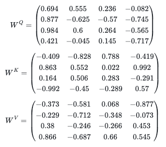
We can create them by sampling a uniform distribution from -1 to 1:
W_Q = np.random.uniform(-1, 1, size=(4, 4))
W_K = np.random.uniform(-1, 1, size=(4, 4))
W_V = np.random.uniform(-1, 1, size=(4, 4))
Let’s create an abstraction to store our weight matrices so that we can use them later.
class W_matrices:
    def __init__(self, n_lines, n_cols):
        self.W_Q = np.random.uniform(low=-1, high=1, size=(n_lines, n_cols))
        self.W_K = np.random.uniform(low=-1, high=1, size=(n_lines, n_cols))
        self.W_V = np.random.uniform(low=-1, high=1, size=(n_lines, n_cols))
def print_W_matrices(self):
print(‘W_Q : \n’, self.W_Q)
print(‘W_K : \n’, self.W_K)
print(‘W_V : \n’, self.W_V)
After the multiplication with input X, we get:
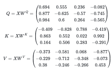
Q = np.matmul(X_example, W_Q)
K = np.matmul(X_example, W_K)
V = np.matmul(X_example, W_V)
The next step is to (dot) multiply the query and key matrices to produce the attention scores. As discussed above, the resulting matrix is a result of the dot products (similarity) between every pair of vectors in the Q and K sets:
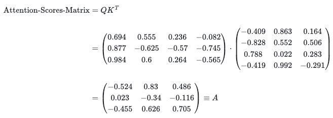
Attention_scores = np.matmul(Q, np.transpose(K))
We stress once again that, essentially, the attention scores represent the proximity of vectors in space. That is to say, for two normalized vectors, the more their dot product gets to 1, the closer they are to each other. It also means that the words are closer to each other. So, this way, the model takes into account the measure of proximity of words from the context of the sentence they appear in.
Then the matrix A is divided by the square root of 4. This operation intends to avoid the problem of vanishing/exploding gradients. It emerges here due to the fact that two vectors of dimension d_k, whose components are distributed randomly with 0 mean and standard deviation 1, produce a scalar product that has also 0 mean but standard deviation d_k. Since the next step involves the exponentiation of these scalar product values, this implies that for some values there would be huge factors like exp(d_k) (consider the fact that the actual dimension used in the paper is 512). For others, there would be very small ones like exp(−d_k).
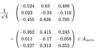
Attention_scores = Attention_scores / 2
We are now ready to apply the softmax map:

where x_i is the i-th component of a generic vector. Thus, it results in a distribution of probabilities. It is worth mentioning that this function is defined only for vectors, not for 2-dimensional matrices. When it is said that softmax is applied to A_norm, in reality, softmax is applied separately to each row (vector) of A_norm. It assumes a format of a stack of 1-dimensional vectors representing the weights for each vector in V. It means that operations that are typically applied to matrices, like rotations, don’t make sense in this context. This is because we are not dealing with a cohesive 2-dimensional entity, but rather a collection of separate vectors that just happen to be arranged in a 2-dimensional format.

Softmax_Attention_Matrix = np.apply_along_axis(softmax, 1, Attention_scores)
Our result is then multiplied by V and we arrive at the one-head attention matrix which is an updated version of the initial V’s (and also the initial X’s):
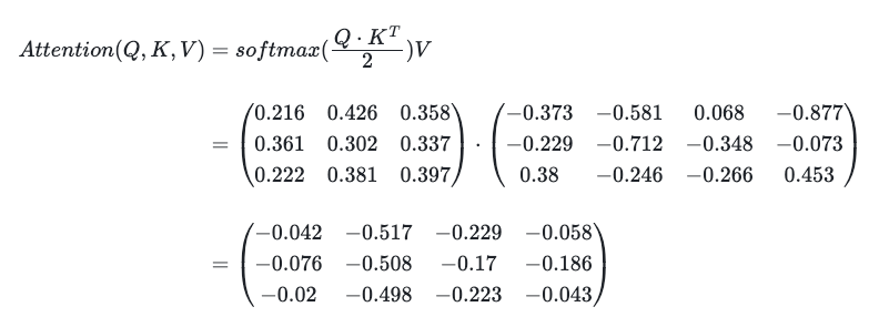
One_Head_Attention = np.matmul(Softmax_Attention_Matrix,V)
Let’s now build a class that initializes our weight matrices and implements a method to compute a single-head attention layer. Notice that we are only concerned about the forward pass, so methods such as backpropagation will be discussed in an upcoming article.
class One_Head_Attention:
    def __init__(self, d_model, X):
        self.d_model = d_model
        self.W_mat = W_matrices(d_model, d_model)

        self.Q = np.matmul(X, self.W_mat.W_Q)
        self.K = np.matmul(X, self.W_mat.W_K)
        self.V = np.matmul(X, self.W_mat.W_V)

    def print_QKV(self):
        print('Q : \n', self.Q)
        print('K : \n', self.K)
        print('V : \n', self.V)


    def compute_1_head_attention(self):
        Attention_scores = np.matmul(self.Q, np.transpose(self.K))
        print('Attention_scores before normalization : \n', Attention_scores)
        Attention_scores = Attention_scores / np.sqrt(self.d_model)
        print('Attention scores after Renormalization: \n ', Attention_scores)
        Softmax_Attention_Matrix = np.apply_along_axis(softmax, 1, Attention_scores)
        print('result after softmax: \n', Softmax_Attention_Matrix)
        # print('Softmax shape: ', Softmax_Attention_Matrix.shape)

        result = np.matmul(Softmax_Attention_Matrix, self.V)
        print('softmax result multiplied by V: \n', result)

        return result

    def _backprop(self):
        # do smth to update W_mat
        pass
The Multi-Head Attention Layer
The paper defines multi-head attention as the application of this mechanism ℎ times in parallel, each one with its own W^Q, W^K and W^V matrices. At the end of the procedure, one has ℎ self-attention matrices, called heads:

where Q_i, K_i, V_i are defined by multiplication of their respective weight matrices W_i^Q, W_i^K and W_i^V. In our example, we already have one single-head attention calculated:


The residual connection prevents the model from running into a vanishing/exploding gradient problem (again). The main idea is that when we add the original X vector to the result of the matrix multiplication, the norm of each final vector is resized to be of the same order of magnitude as the original one.
By this procedure, one maps 3 4-dimensional vectors (X’s) into another pack of 3 4-dimensional vectors (updated V’s). What is the gain, then? The answer is that now we have 3 vectors that somehow encode (and this encoding gets better as long training takes place) the attention/semantic relations between the words occurring in the sentence contrasting with the 3 initial vectors that were written down by the simple one-hot encoding algorithm. That is to say, now we have an embedding of such vectors that takes into account the context in which they appear in a much more refined way.
Let’s implement the multi-head attention layer as a new class:
class Multi_Head_Attention:
    def __init__(self, n_heads, d_model, X):
        self.d_model = d_model
        self.n_heads = n_heads
        self.d_concat = self.d_model*self.n_heads # 4*8
        self.W_0 = np.random.uniform(-1, 1, size=(self.d_concat, self.d_model))
        # print('W_0 shape : ', self.W_0.shape)
        self.heads = []
        self.heads_results = []
        i = 0
        while i < self.n_heads:
            self.heads.append(One_Head_Attention(self.d_model, X))
            i += 1

    def print_W_0(self):
        print('W_0 : \n', self.W_0)

    def print_QKV_each_head(self):
        i = 0
        while i < self.n_heads:
            print(f'Head {i}: \n')
            self.heads[i].print_QKV()
            i += 1

    def print_W_matrices_each_head(self):
        i = 0
        while i < self.n_heads:
            print(f'Head {i}: \n')
            self.heads[i].W_mat.print_W_matrices()
            i += 1

    def compute(self):
        for head in self.heads:
            self.heads_results.append(head.compute_1_head_attention())
            # print('head: ', self.heads_results[-1].shape)

        multi_head_results = np.concatenate(self.heads_results, axis=1)
        # print('multi_head_results shape = ', multi_head_results.shape)

        V_updated = np.matmul(multi_head_results, self.W_0)
        return V_updated

    def back_propagate(self):
        # backpropagate W_0
        # call _backprop for each head
        pass
Positional Encoding and Fully Connected Feed-Forward Network
We have covered what we consider to be the core of the paper “Attention is all you need” regarding the encoder part. There are 2 important pieces that we left out and will discuss in this section. The first is presented at the very beginning of the encoder stack, namely, the positional encoding procedure.
For the sake of simplicity, the way we input the vectors into the attention mechanism does not consider the order of the words that appear in the sentence. This is indeed a major drawback. It is evident that the order of words is a crucial element of their semantic value, and so, it must be present in the embeddings. In the paper, the authors propose a solution to this problem by making use of sine and cosine functions. They are used to encode the order in every component of the embedding vectors. For a word that occurs at the i-th position in the sentence, each of its j-th component is associated with the positional encoding as follows:

and, since PE_i is a vector of the same size as the embedding vectors, it is added to them to include the positional information the word assumes in the sentence:

One great advantage of using this construction resides in the fact we have included new information without requiring any further space. Another one is that the information is spread over the whole vector and consequently, it communicates with all the other components of the other vectors through the many matrix multiplications occurring in the layers.
We are now ready to implement our positional encoding layer:
class Positional_Encoding:
    def __init__(self, X):
        self.PE_shape = X.shape
        self.PE = np.empty(self.PE_shape)
        self.d_model = self.PE_shape[1]

    def compute(self, X):
        for i in range(self.PE_shape[0]):
            for j in range(self.PE_shape[1]):
                self.PE[i,2*j] = math.sin(i/(10000**(2*j/self.d_model)))
                self.PE[i,2*j+1] = math.cos(i/(10000**(2*j/self.d_model)))
                # this way we are assuming that the vectors are ordered stacked in X

        return X + self.PE
Finally, at the end of the encoder, there is a simple fully connected feed-forward network consisting of 2 layers. Albeit it is not an innovative part of the paper, it plays an important role in adding nonlinearity through the ReLu activation functions and, as a result, capturing other semantic associations [2].
Let’s implement them:
class FFN:
    def __init__(self, V_updated, layer1_sz, layer2_sz):
        self.layer1_sz = layer1_sz
        self.layer2_sz = layer2_sz
        self.layer1_weights = np.random.uniform(low=-1, high=1, size=(V_updated.shape[1], layer1_sz))
        self.layer2_weights = np.random.uniform(low=-1, high=1, size=(layer2_sz, V_updated.shape[1]))

    def compute(self, V_updated):
        result = np.matmul(V_updated, self.layer1_weights)
        result = np.matmul(result, self.layer2_weights)

        return result

    def backpropagate_ffn(self):
        pass
Conclusions
We started by exploring the concept of embeddings in NLP, explaining how words and their semantic meanings are translated into numerical forms that AI models can process. We then delved into the Transformer architecture, starting with the Single-Head Attention layer and explaining the roles of Queries, Keys, and Values in this framework.
We then covered the Attention Scores, what they represent, and how to normalize them in order to address the challenges of vanishing and exploding gradients. After guiding the understanding of how a Single-Head Attention layer works, we went through the process of creating a Multi-Head Attention mechanism. It allows the model to process and integrate multiple perspectives of input data simultaneously.
As a final component, we covered Positional Encoding and the simple fully connected feed-forward network. The first allows us to preserve the order of words, which is key to understanding the contextual meaning of sentences. The second plays the important role of adding nonlinearity through the activation functions.
Keep in touch: LinkedIn, X/Twitter, Medium.
References
[1] Ashish Vaswani et al. (2017), Attention is all you need https://doi.org/10.48550/arXiv.1706.03762
[2] Mor Geva, et al. (2022). Transformer Feed-Forward Layers Build Predictions by Promoting Concepts in the Vocabulary Space, Proceedings of the 2022 Conference on Empirical Methods in Natural Language Processing, 30–45 https://arxiv.org/pdf/2203.14680.pdf
More articles: https://zaai.ai/lab/

