JEPA for time series: a labeled-budget stress test

Introduction

A national statistics agency does not publish one forecast. The public Labour collection built from the Australian Bureau of Statistics' monthly employment survey is a 57-series hierarchy split by region, gender and employment status.

A retailer or a utility with a modest footprint faces the same problem at a larger scale: one forecasting model per store, per meter, per SKU, each one wrong in its own way before a stock-out or a staffing shortfall follows. Training every one of those well, especially the series with only a few years of usable history, is the setting self-supervised pretraining exists to help with.

The standard recipe pretrains an encoder to reconstruct the values under a mask, the time-series analogue of a masked autoencoder. A newer family predicts the masked region's representation instead of its raw values: the Joint-Embedding Predictive Architecture (JEPA), proposed by LeCun [1] and demonstrated on images by Assran et al. [2] (I-JEPA) and on video by Bardes et al. [3] (V-JEPA).

On images, He et al.'s masked-autoencoder ablation [4] shows the two kinds of objective can rank differently depending on how the encoder is evaluated. One that scores badly under a frozen linear probe can still score well once the whole model is fine-tuned.

JEPA has already reached time series. Ennadir et al.'s TS-JEPA [5] adapts it there, motivated by the same idea, that reconstruction can be vulnerable to noise a latent target can ignore, and reports it matching or surpassing state-of-the-art baselines on classification and forecasting benchmarks. Verdenius et al.'s LaT-PFN [6] uses the same latent-prediction idea for in-context time-series forecasting. We could not find a matched-encoder comparison of the two objectives in either, or a sweep of how much labeled data the downstream head needs before the choice stops mattering.

In this article, we build a small JEPA that runs on a public panel, pretrain a matched reconstruction baseline from the same encoder and masking scheme, and add a random-features floor and a from-scratch control. We sweep the one variable a practitioner actually controls: how many labeled forecasting examples the downstream head gets to see, from a handful per series to the whole pretraining pool.

On this panel, the two pretraining objectives score the same at every labeled budget we tried, which does not obviously follow from TS-JEPA's own motivating claim that latent prediction should handle noise better than reconstruction. What separates a good forecaster from a bad one is whether the encoder was pretrained at all, and a compute-matched control rules out extra training steps as the explanation.

A separate experiment then asks which piece of JEPA's collapse-prevention machinery is doing that work, and finds that the stop-gradient carries JEPA's stability while the EMA target is a smaller refinement. A training-loss curve hides the damage of losing the stop-gradient entirely, a rank diagnostic understates it, and only a downstream probe shows its full size. As always, the code is available on our GitHub.

Latent prediction versus value reconstruction

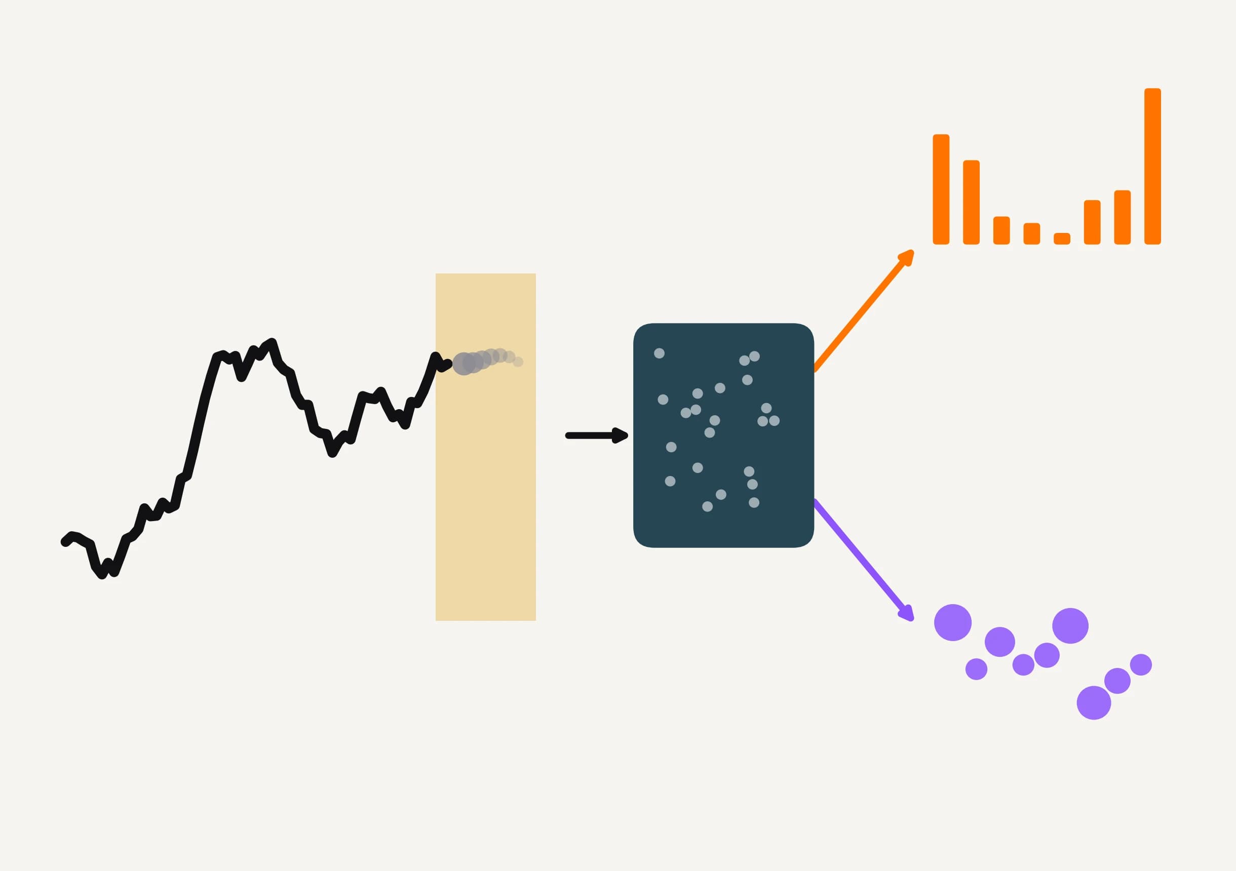
Self-supervised pretraining for time series usually means masking part of a window and asking the encoder to fill it back in, the way a masked autoencoder scores itself by how well a decoder reconstructs the exact values underneath the mask. JEPA scores it differently: instead of reconstructing the masked values, a predictor guesses their representation, the vector a second encoder assigns to them, and the comparison happens in that vector space rather than in value space.

Figure 1 shows one context window from a series we use later in this article, employment among full-time male workers in New South Wales. We mask the next eight months and ask two different models to explain them. A reconstruction model must recover the eight exact counts, a one-off data revision or a rounding artifact included: whatever is under the mask is the target it is scored against. A latent-prediction model only has to match a summary a target encoder computes from those same eight months, free to have already discarded the kind of detail a forecast does not need.

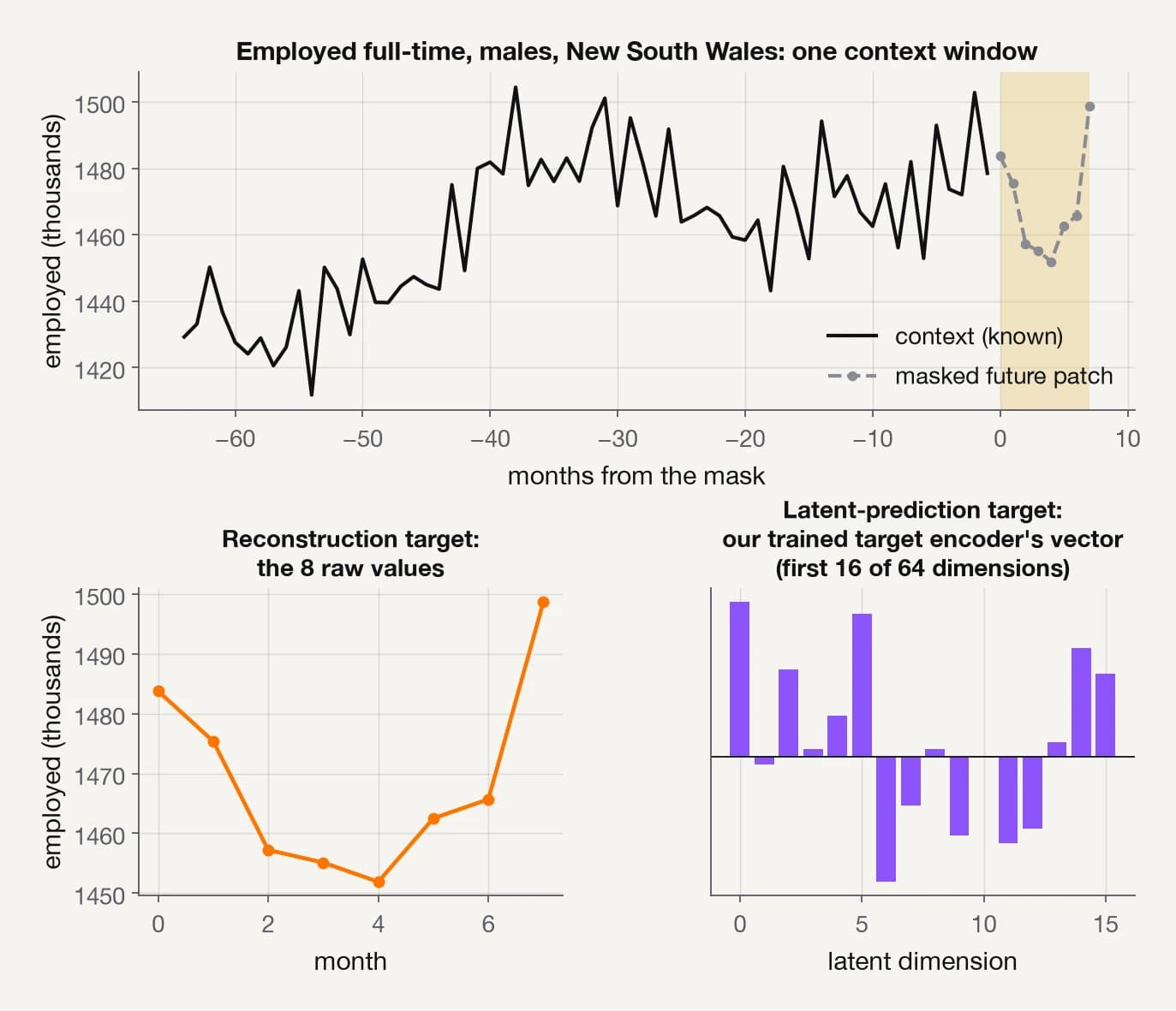
The reconstruction target is fixed: it is simply the data, and it never moves during training. The latent-prediction target moves instead, since it is the output of another encoder that is itself changing while the online encoder trains, and that opens a shortcut reconstruction does not have. Both encoders can collapse to outputting the same constant for every input, and the loss falls to zero without the model learning anything about the series. That shortcut is what we guard against in the next section.

A minimal JEPA for time series

We built a small JEPA for this comparison, a 68,000-parameter encoder that pretrains in under a minute on CPU, using one shared, channel-independent patch encoder for every series, in the spirit of PatchTST [7]. A single set of weights processes one series' window at a time, so the 57 series in our panel train one encoder rather than 57.

We split each window into 8-step patches, normalize each window by the mean and standard deviation of its own context, and denormalize again before scoring. The target shares the context's own statistics, so nothing about the future patch leaks into its own scale. This patch encoder is a small transformer, the same architecture underneath every arm in this article:

class PatchEncoder(nn.Module):
    """One shared encoder: each series' window is one example."""
    def __init__(self, n_positions=9):
        super().__init__()
        self.patch_embed = nn.Linear(PATCH_LEN, D_MODEL)
        self.pos_embed = nn.Parameter(torch.randn(n_positions, D_MODEL) * 0.02)
        layer = nn.TransformerEncoderLayer(
            d_model=D_MODEL, nhead=4, dim_feedforward=128,
            dropout=0.1, batch_first=True, activation="gelu",
        )
        self.encoder = nn.TransformerEncoder(layer, num_layers=2)

    def forward(self, patches):
        x = self.patch_embed(patches) + self.pos_embed[: patches.shape[1]]
        return self.encoder(x)

We add two more pieces on top of that shared encoder for the JEPA head, shown in Figure 2. An exponential moving average (EMA) target encoder is a copy of the online encoder. Its weights are updated by an exponential moving average of the online weights, never by its own gradient, following the recipe BYOL [8] popularized for images.

The target encoder processes the full window, context patches and the future patch together, and the representation it assigns to the future patch is the prediction target. A small predictor then takes the context patches' representations, plus a learnable token marking the future patch's position, and tries to match that target. The target's own gradient is blocked, so only the predictor and the online encoder are pushed to change:

ctx_latents = encoder(ctx)                      # online path, gradients flow
with torch.no_grad():
    full_latents = target_encoder(full_patches)  # EMA copy, no gradients
target_latent = full_latents[:, -1, :].detach()  # stop-gradient
pred = predictor(ctx_latents)                    # predictor sees context only
loss = F.mse_loss(pred, target_latent)
...
target_encoder.update(encoder)                   # EMA step, after the optimizer step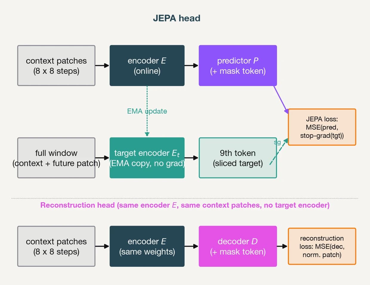

These are two separate mechanisms, the EMA update and the stop-gradient. Later in this article we test what each one is doing, and find that BYOL's and SimSiam's readings of their necessity do not simply agree. A third family of methods, VICReg [9], prevents collapse differently again, by directly penalizing low variance and high covariance; we do not use it here.

The reconstruction head reuses the identical encoder and context patches we just described. It has no target encoder. A small decoder maps the context representations, plus the same kind of position token, directly to the eight values of the future patch on the context's normalized scale. The loss is mean squared error against those same values:

ctx_latents = encoder(ctx)         # same encoder, same context patches
pred_values = decoder(ctx_latents) # decodes to 8 values, no target encoder
loss = F.mse_loss(pred_values, true_future_patch)

Everything else, the encoder, the patch size, the masking scheme, is shared between the two arms on purpose. The only thing that differs between them is what the loss is scored against.

JEPA in practice

Dataset and protocol

We use the Labour collection [10], monthly Australian employment counts published by the Australian Bureau of Statistics and distributed for forecasting research through Nixtla's datasetsforecast package. The panel is a small hierarchy of 57 series: a national total, 8 states, 16 state-by-gender series and 32 bottom-level series split by region, gender and employment status (for example, full-time employed men in New South Wales).

Twenty-five of the 57 series are exact sums of the other 32. We treat every series independently and do not use the hierarchy's structure, but we return to this fact below, because it matters for how confidently we can read the headline result:

from datasetsforecast.hierarchical import HierarchicalData

Y_df, _, _ = HierarchicalData.load("data", "Labour")

Each series runs from February 1978 to December 2019, 503 months in total.

We hold out the last 8 months of every series as the test horizon. The 24 months before that form three validation windows per series, used only to pick a checkpoint, and the remaining 471 months are available for both pretraining and downstream training.

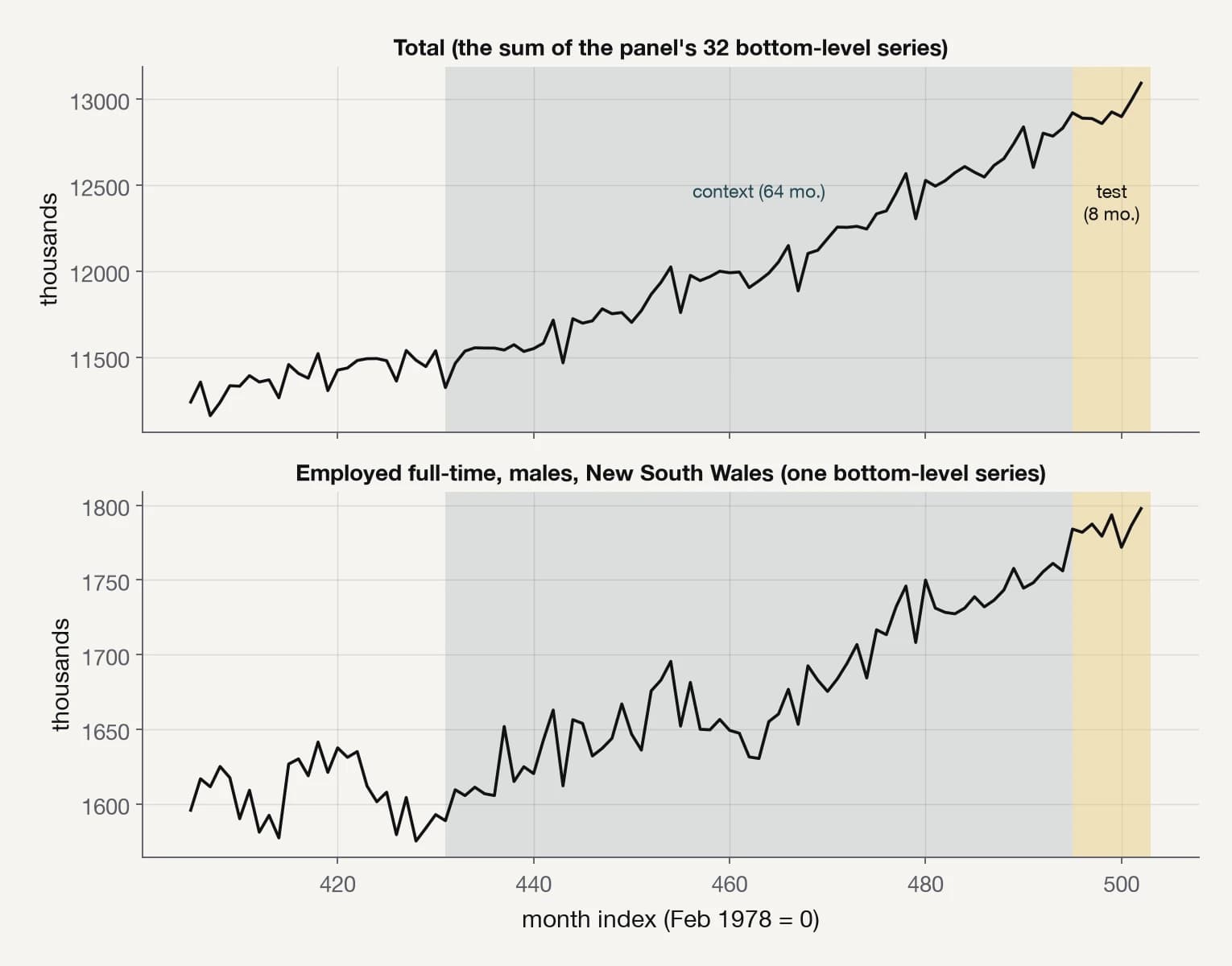
Figure 3 shows two of the 57 series over their last few years, the aggregate Total and one bottom-level series, with the context window and the test horizon marked.

We split each context window, 64 months, into 8 patches of 8 steps each. The future patch we mask, or forecast, is exactly one more patch, so the same block JEPA learns to predict in latent space is the block the downstream head has to forecast in value space.

We pretrain both objectives for 1,500 steps on every window inside the 471-month region, about 400 windows per series. We then evaluate each pretrained encoder two ways: as a frozen probe, where only a linear head trains on top of the encoder, and fine-tuned, where the encoder and the head train together. Six arms in total:

• JEPA, frozen probe and fine-tuned
• Reconstruction, frozen probe and fine-tuned
• Scratch: the same architecture trained end to end with no pretraining
• Random-frozen: a frozen probe on a never-trained encoder, the floor that tells us whether pretraining does anything at all

The downstream head, a single linear layer over the mean-pooled context representations, is restricted to a budget of k of the pretraining pool's own windows, with their true future values attached, sampled per series:

def sample_labeled_starts(uids, pretrain_starts, k, seed):
    labeled = {}
    for i, uid in enumerate(uids):
        avail = pretrain_starts[uid]
        rng = np.random.default_rng(seed * 100003 + i)
        labeled[uid] = rng.choice(avail, size=min(k, len(avail)), replace=False)
    return labeled

k ranges from 4 to 400 windows per series, from about 1 percent of the pretraining pool to all of it. Every trained arm, at every budget, selects its checkpoint by the lowest mean absolute error over the three validation windows, under the same step budget. The rule weighs the panel's large aggregate series most heavily, but it applies equally to every arm.

We score the held-out forecast with the Mean Absolute Scaled Error (MASE) [11, 12], each series' error divided by that same series' own naive-forecast error from a year back, measured on its training history.

A MASE of 1.0 means the model's test error equals that in-sample reference. It does not mean a seasonal-naive forecast would score 1.0 on the test window itself. Actually forecasting this panel's held-out months with the seasonal-naive method scores a mean MASE of 1.36, which is the number we compare against below.

Results

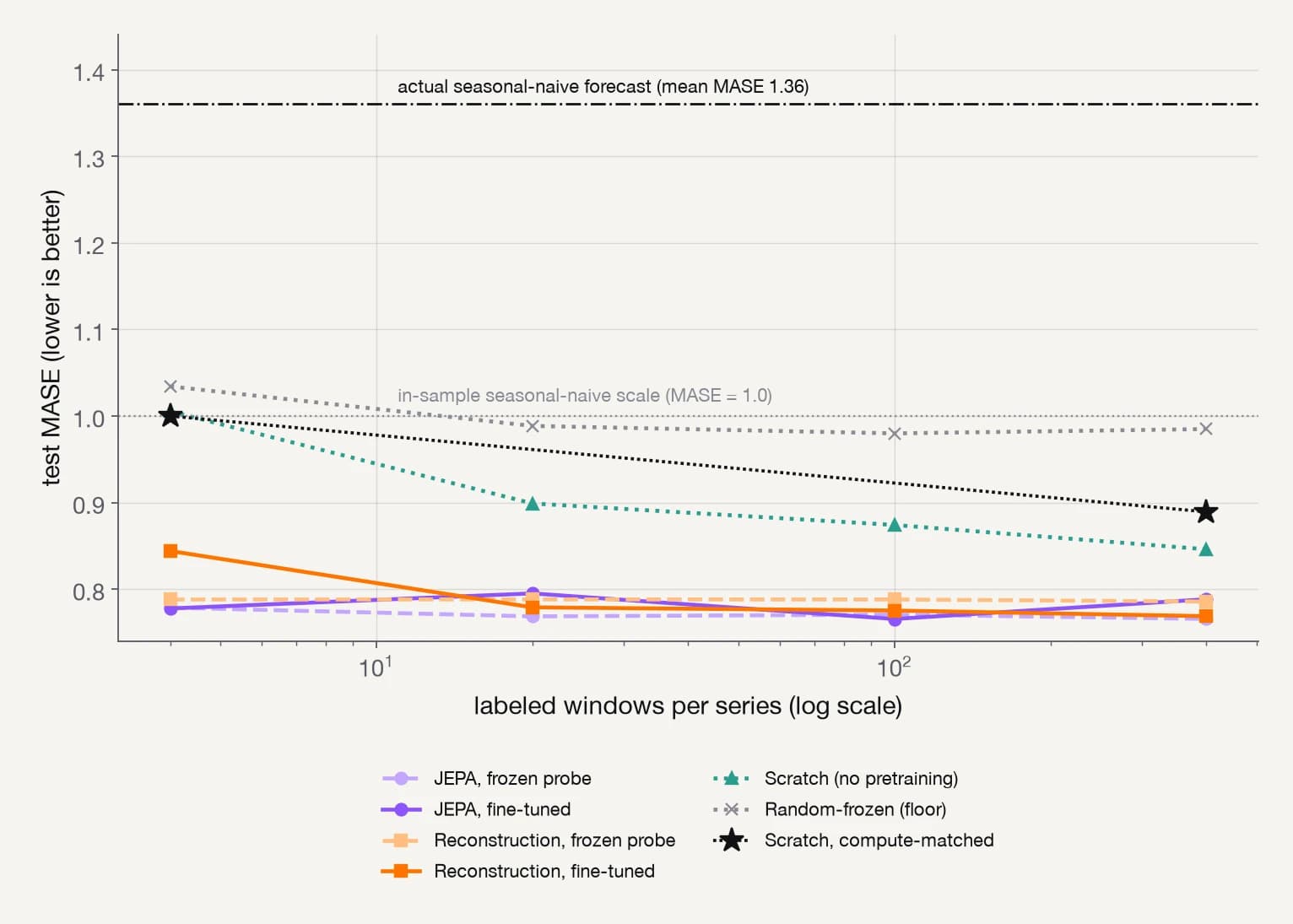
Figure 4 sweeps the labeled budget against test MASE, one line per arm. Two reference lines mark the in-sample scale MASE divides by (1.0) and the seasonal-naive method's own score if actually used to forecast the test window (1.36). JEPA's frozen probe and the reconstruction frozen probe sit on top of each other at every budget. Both pretrained arms sit well below Scratch and Random-frozen, and every arm beats the real seasonal-naive forecast comfortably.

Pooling the three seeds into per-series paired comparisons gives 171 pairs across 57 series. Twenty-five of those series are sums of the other 32, so the comparisons are not fully independent. Splitting the panel by hierarchy level gives the same answer at both levels, which is the strongest check available for the null result below.

JEPA's frozen probe beats reconstruction's frozen probe on 47 to 52 percent of comparisons across the four budgets we tested, straddling half with no trend, indistinguishable from a coin flip. The mean paired difference is 0.01 to 0.02 MASE, against a series-to-series spread of about 0.20, roughly a tenth the size. We ran no significance test on this, but a difference that small next to that spread is not one we would act on.

On this dataset, at this scale, the choice between reconstructing values and predicting their representation does not decide the outcome. That does not obviously follow from TS-JEPA's own motivating claim that latent prediction should handle noise better than reconstruction, and it is not the result we expected going in. We think it is worth reporting plainly rather than reframing it.

Pretraining itself does decide the outcome, and this is also why the pretrained lines in Figure 4 are flat rather than rising with the labeled budget. In forecasting, a window's own future is already known once it is in history. Both pretraining objectives already train on the true next eight months for every window in the pool.

The labeled-budget axis restricts only how many of those windows the downstream head itself is allowed to fit against. Its encoder has already seen all of them. That is also why fine-tuning changes so little for either pretrained arm, at every budget but one: fine-tuning reconstruction's whole encoder on just 4 labeled windows per series makes it worse, not better (0.844 against its own frozen probe's 0.788). That is the signature of overfitting an entire encoder to too little data.

The cleanest evidence for that reading is Scratch at the largest budget, where it sees exactly the same windows the pretrained encoders did. It still loses: 0.846 mean MASE against jepa_frozen's 0.766, on 60 percent of paired comparisons.

Giving Scratch the same number of extra gradient steps that JEPA's pretraining used does not close the gap either. At the smallest budget the compute-matched control lands on 1.000, a coin flip against plain Scratch's own 1.006. At the largest budget it lands on 0.889, slightly worse than plain Scratch's 0.846. Training longer on the same windows is not a substitute for whatever the pretrained encoders extracted from seeing every window's outcome together.

We found that most series in every pretrained arm beat the real seasonal-naive forecast: 82 to 84 percent of series-seed-budget cells for JEPA and reconstruction, pooled across all four budgets, against 77 percent for Scratch and 76 percent for Random-frozen.

Not every series does, for any arm. With only 57 series to learn from, some are always going to be harder than a naive forecast can fix, whichever pretraining objective is used.

The EMA target encoder and the stop-gradient

JEPA needs at least one mechanism to stop the online and target encoders from agreeing on a constant. The usual recipe keeps two. An EMA target encoder moves too slowly for the online encoder to chase into a trivial agreement, and the stop-gradient stops the loss from being reduced by moving the target toward the prediction rather than the other way around.

BYOL's own ablation [8] shows collapse once the EMA decay is pushed to zero, which reads as evidence that the moving target is necessary. SimSiam [13], built for images but in the same family of methods, reports the opposite: the online encoder's own weights, with no momentum copy, are enough, provided the stop-gradient stays in place.

Later theoretical work [14] argues that the EMA target's necessity depends on the predictor's own learning-rate dynamics relative to the encoder, not on the momentum update by itself. That points toward the SimSiam reading without fully closing the question. We test it in the time-series setting, with a downstream probe rather than an image benchmark.

We pretrained three configurations of the JEPA head, which we call cells, for 1,500 steps each, across the same three seeds as the main sweep. Each cell removes one more mechanism than the one above it, so the clean single-variable contrast is no_ema against no_stopgrad, not the full recipe against either one directly:

if cell == "full":
    full_latents = target_encoder(full_patches)      # EMA copy, no grad
elif cell == "no_ema":
    full_latents = encoder(full_patches).detach()    # same weights, stop-grad kept
elif cell == "no_stopgrad":
    full_latents = encoder(full_patches)              # same weights, grad flows

Figure 5 tracks three things per cell, averaged over the three seeds: the training loss, the effective rank of the context representation, and the mean norm of the target vector the loss is scored against.

Effective rank (Roy & Vetterli, 2007 [15]) summarizes how many independent directions a batch of representations actually uses. With 64 latent dimensions, a value near 1 would mean every window maps to nearly the same point, and a value near 64 would mean the encoder uses the full space.

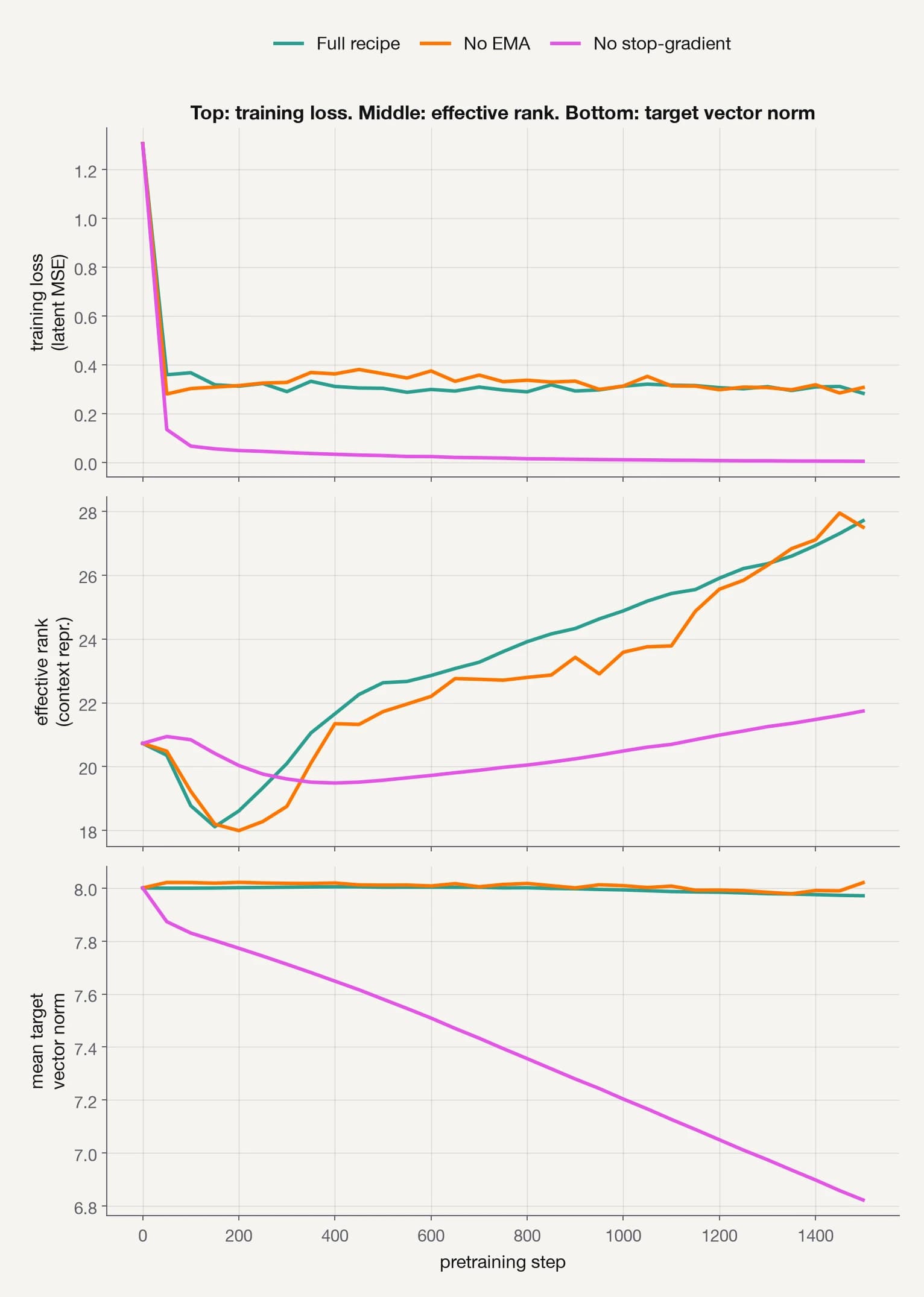
Removing the stop-gradient collapses the training loss to a small fraction of the two healthy cells' level. That is exactly the signature a practitioner watching only a loss curve would read as the best run of the three.

Effective rank moves too, but by much less than the loss implies. By the end of training, the collapsing cell's context-representation rank reaches about 22, against about 27.5 for the two healthy cells, a real, seed-consistent gap of roughly 20 percent next to a training loss that is around sixty times smaller. Measuring rank a second way, directly on the target-slot representation the loss acts on, shows an even smaller gap between the cells.

The target vector's own norm explains part of why the loss is so misleading. It shrinks by about 15 percent over training for the collapsing cell, while the two healthy cells hold flat. Part of the loss reduction is a smaller target, not a better prediction: the ruler got shorter, the aim did not improve.

The downstream frozen probe, run at the smallest labeled budget from the main sweep (k=4, comparable to jepa_frozen's 0.779 there), is what finally shows the full damage. It reads 0.78 MASE for the full recipe, 0.81 for no EMA, and 1.22 for no stop-gradient, about 56 percent worse, a gap that holds in every one of the three seeds.

The EMA-only gap does not hold as clearly. It averages small and is not even consistent in direction from seed to seed. At this scale, the stop-gradient carries JEPA's stability and the EMA target is a smaller refinement. The loss curve would have hidden that entirely, and both rank readouts understated it. Only the downstream probe shows how large the gap really is.

Conclusion

On a public monthly panel, predicting the future in latent space and reconstructing it in value space produced forecasters that were indistinguishable from each other at every labeled budget we tested. That is a null result, not the crossover we set out to find.

What separated a good forecaster from a bad one was whether the encoder had been pretrained at all, and specifically whether it had already seen every window's outcome during pretraining. Both objectives beat a from-scratch model and a random-features floor, most clearly when the downstream head's own labeled budget was small. A compute-matched control ruled out extra gradient steps as the explanation, at both the smallest and the largest budget we tried.

Nonetheless, several choices bound how far this null result should generalize. The panel is small (57 series, well under 30,000 raw observations) and so is the encoder, pretrained for minutes on CPU rather than on the schedules foundation-model papers use.

The masking ratio, one patch in nine, is also far below what image JEPA and MAE work uses. Asking two objectives to explain an already mostly visible window may be exactly the regime in which they are expected to agree. A larger panel, a bigger encoder, or a harder masking ratio could separate the two objectives where this one could not.

We trust the collapse decomposition's stop-gradient finding specifically, because it holds in every one of three seeds by a wide margin, while the EMA target's own cost is small and not even consistent in direction from seed to seed. The training-loss curve alone would have hidden the damage entirely, and an effective-rank readout, on the pooled context representation or on the exact tensor the loss collapses, would have understated it. Only the downstream probe showed its full size.

We recommend spending the engineering budget on pretraining at all, on whichever objective is easiest to implement correctly, before spending it on the choice between reconstruction and latent prediction. We would also verify any from-scratch JEPA implementation with a downstream probe, rather than trusting the training loss or a rank diagnostic by themselves.

References

[1] LeCun, Y. (2022). A Path Towards Autonomous Machine Intelligence. OpenReview. https://openreview.net/forum?id=BZ5a1r-kVsf

[2] Assran, M., Duval, Q., Misra, I., Bojanowski, P., Vincent, P., Rabbat, M., LeCun, Y., & Ballas, N. (2023). Self-Supervised Learning from Images with a Joint-Embedding Predictive Architecture. arXiv:2301.08243. https://arxiv.org/abs/2301.08243

[3] Bardes, A., Garrido, Q., Ponce, J., Chen, X., Rabbat, M., LeCun, Y., Assran, M., & Ballas, N. (2024). Revisiting Feature Prediction for Learning Visual Representations from Video. arXiv:2404.08471. https://arxiv.org/abs/2404.08471

[4] He, K., Chen, X., Xie, S., Li, Y., Dollár, P., & Girshick, R. (2022). Masked Autoencoders Are Scalable Vision Learners. arXiv:2111.06377. https://arxiv.org/abs/2111.06377

[5] Ennadir, S., Golkar, S., & Sarra, L. (2025). Joint Embeddings Go Temporal. arXiv:2509.25449. https://arxiv.org/abs/2509.25449

[6] Verdenius, S., Zerio, A., & Wang, R. L. M. (2024). LaT-PFN: A Joint Embedding Predictive Architecture for In-context Time-series Forecasting. arXiv:2405.10093. https://arxiv.org/abs/2405.10093

[7] Nie, Y., Nguyen, N. H., Sinthong, P., & Kalagnanam, J. (2023). A Time Series is Worth 64 Words: Long-Term Forecasting with Transformers. arXiv:2211.14730. https://arxiv.org/abs/2211.14730

[8] Grill, J.-B., Strub, F., Altché, F., Tallec, C., Richemond, P. H., Buchatskaya, E., Doersch, C., Pires, B. A., Guo, Z. D., Azar, M. G., Piot, B., Kavukcuoglu, K., Munos, R., & Valko, M. (2020). Bootstrap Your Own Latent: A New Approach to Self-Supervised Learning. arXiv:2006.07733. https://arxiv.org/abs/2006.07733

[9] Bardes, A., Ponce, J., & LeCun, Y. (2022). VICReg: Variance-Invariance-Covariance Regularization for Self-Supervised Learning. arXiv:2105.04906. https://arxiv.org/abs/2105.04906

[10] Australian Bureau of Statistics. Labour Force, Australia. Distributed for forecasting research via Nixtla's datasetsforecast package. https://github.com/Nixtla/datasetsforecast

[11] Hyndman, R. J., & Koehler, A. B. (2006). Another look at measures of forecast accuracy. International Journal of Forecasting, 22(4), 679-688.

[12] Makridakis, S., Spiliotis, E., & Assimakopoulos, V. (2020). The M4 Competition: 100,000 time series and 61 forecasting methods. International Journal of Forecasting, 36(1), 54-74.

[13] Chen, X., & He, K. (2021). Exploring Simple Siamese Representation Learning. arXiv:2011.10566. https://arxiv.org/abs/2011.10566

[14] Tian, Y., Chen, X., & Ganguli, S. (2021). Understanding Self-Supervised Learning Dynamics without Contrastive Pairs. arXiv:2102.06810. https://arxiv.org/abs/2102.06810

[15] Roy, O., & Vetterli, M. (2007). The effective rank: A measure of effective dimensionality. EUSIPCO 2007.